Warsaw Public Transport Analysis for Pizza Brand Expansion

By Sasha Fridman, March 2025

---

image.png

📖 Project Description

👁️ Project Overview

The goal of this project is to analyze Warsaw’s public transportation network to help a global pizza brand identify optimal locations for opening new pizzerias. We aim to identify the busiest transport hubs - areas with high passenger flow. We will independently source the necessary data (as no specific data is available at the start).

Note 1: The focus will be primarily on non-central stations (as their popularity and traffic are evident), though we may include central stations in our analysis as well.
Note 2: Public transport will be the main focus of this study (being one of the layers in decision-making for opening new pizza locations). Additionally, we may complement the analysis with other types of people flows, such as private car traffic, if reliable data is available.

📋 Project Terminology and Notations

• Key terms. To ensure clarity in our analysis, we will define several key terms upfront:

  • Geospatial data - in general, is information that has a geographic component and can be linked to specific locations on the Earth’s surface (for instance, details about places, addresses, and coordinates). In current project we mostly refer to geospatial data as for coordinates - latitude and longitude of data points like transport stops.
  • GTFS dataset - GTFS (General Transit Feed Specification) is a standardized format for sharing data about public transit schedules, which in fact is a set of related files zipped together.
  • Headway - time between vehicle departures, in other words it’s wait time. Headway is applicable for routes with frequency-based scheduling.
  • Weighted Trips Capacity - a metric that estimates passenger flows at each stop by accounting for both the number of public transport trips and the passenger capacity of each transport type. Simply counting raw trips would be misleading, so trips are adjusted based on transport capacity. For example, a bus (base unit) has a weight of 1 (~ 90 passengers), while a tram has a weight of 2.2 (~200 passengers). This approach provides a more accurate impact calculations for different transport types on passenger flows across stops.

• Symbols. There are also several symbols we use in the project to highlight key points:

  • 💡 - An important insight relevant to this specific part of the study.
    

  • 💡💡 - A key insight with significant implications for the entire project.
    

  • ⚠ - Information requiring special attention (e.g., major clarifications, major conclusions or decision explanations), as it may impact further analysis.

    Additional clarifications with more local relevance are preceded by the bold word “Note” and/or highlighted in italics.**

📋 Data Sources and Description

1. GTFS Data (warsaw.zip): A dataset providing static information about Warsaw’s public transportation system.

   • agency.txt: Information about the transit agencies managing Warsaw’s public transport (e.g., name, contact details).

   • attributions.txt: Specifies whether an organization is a data producer, operator, or authority.

   • calendar_dates.txt: Information about service availability on special days - exceptions to the standard schedule, such as holidays.

   • feed_info.txt: Metadata about the dataset (e.g., publisher name, website, and feed version).

   • frequencies.txt: Specifies headway (time between vehicle departures) for routes with frequency-based scheduling.

   • routes.txt: Details about the routes served by each transit agency (route ID, name, type).

   • shapes.txt: Describes the exact paths taken by vehicles along a route (latitude, longitude), Essential for visualizing transit flow on a map.

   • stops.txt: Locations of bus stops, tram stops, and metro stations (stop ID, name, latitude, longitude).
     

   • stop_times.txt: Arrival and departure times for each trip at each stop (trip ID, stop ID, arrival time, departure time, stop sequence). This file is the core for our passenger flow analysis.

   • trips.txt: Individual trips along each route (trip ID, route ID, service ID).

   Note 1: The GTFS feed is available at https://mkuran.pl/gtfs/warsaw.zip (maintained by Mikołaj Kuranowski, a developer dedicated to enhancing public transportation data accessibility in Poland). The source of data - Zarząd Transportu Miejskiego (ZTM) also known as Warsaw Public Transport (WTP). Data last updated at January 18, 2025.

   At the time of this study, the official website of Warsaw Public Transport (wtp.waw.pl) was experiencing technical difficulties (403 ERROR - Request Blocked). Thus, we relied on the warsaw.zip dataset from mkuran.pl, which provides sufficient data for analysis.

   Note 2: Since warsaw.zip is ~ 90MB (~ 606 MB after extraction), we use a script to automate downloading and extracting the file when needed (instead of loading it directly when sharing e.g. via GitHub)

   Note 3: While this feed offers comprehensive data on Warsaw’s public transportation system, it doesn’t not include specific data such as passenger counts. In other words it focuses on transit schedules, not real-time passenger load data. However, relying on Warsaw’s transportation management decisions (supported by public reports and citizen surveys), this approach should effectively highlight main traffic spots, which will be sufficient for the current study

   If requested for more precise analysis in the next steps we may access the Warsaw open data portal to gain insight on the online data as well.

📚 Loading Data and Libraries

# data manipulation libraries
import pandas as pd
import numpy as np
import sidetable
import requests
import zipfile
import io
import os

# date and time handling
from datetime import datetime, timedelta

# handling geo-data
%pip install gtfs_kit -q
%pip install geopy -q

# a stable and widely compatible version
%pip install folium==0.17.0 -q 

import gtfs_kit as gk
from gtfs_kit import Feed
from geopy.distance import geodesic

# visualization libraries
import matplotlib.pyplot as plt
import matplotlib.ticker as ticker
from matplotlib.ticker import ScalarFormatter, EngFormatter
import seaborn as sns
import plotly.express as px
import plotly.graph_objects as go
from plotly.subplots import make_subplots
import plotly.io as pio # tools for saving and exporting and visualizations
import folium
from folium.plugins import HeatMap
from folium.plugins import MarkerCluster

# Matplotlib and Seaborn visualization configuration
plt.style.use('seaborn-v0_8')  # more attractive styling
plt.rcParams.update({
    'figure.figsize': (12, 7),  
    'grid.alpha': 0.5,
    'grid.linestyle': '--',
    'font.size': 8,
    'axes.titlesize': 14,
    'axes.labelsize': 10})
sns.set_theme(style="whitegrid", palette="deep")

# Pandas display options
# pd.set_option('display.max_columns', None)
table_width = 150
# pd.set_option('display.width', table_width)
col_width = 40
# pd.set_option('display.max_colwidth', col_width)
# pd.set_option('display.precision', 2)
pd.set_option('display.float_format', '{:.2f}'.format) # displaying normal numbers instead of scientific notation

# Python and Jupyter/IPython utility libraries and settings
import warnings
warnings.filterwarnings('ignore', category=FutureWarning)
warnings.filterwarnings('ignore', category=UserWarning)

from IPython.core.interactiveshell import InteractiveShell
InteractiveShell.ast_node_interactivity = 'all' # notebook enhanced output
from IPython.display import display, HTML, Markdown  # broader options for text formatting and displaying
import textwrap # for formatting and wrapping text (e.g. to manage long strings in outputs)

Note: you may need to restart the kernel to use updated packages.
Note: you may need to restart the kernel to use updated packages.
Note: you may need to restart the kernel to use updated packages.

🚌 Warsaw Public Transport Overview

• Components:
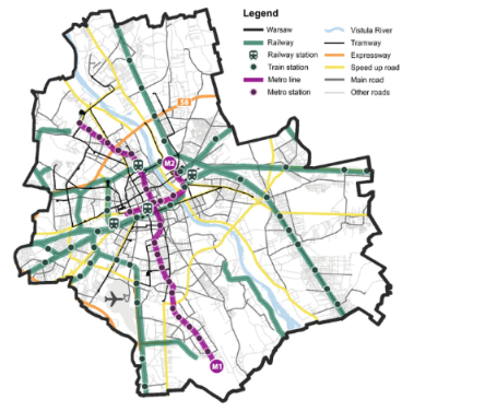
  • Metro (2 lines): As of 2024, the Warsaw Metro comprises two lines (M1 and M2) with a total of 39 stations, covering approximately 41 kilometers.
    
  • Trams (24 lines): The tram network consists of 24 lines, serving 538 stops.
    
  • Buses: The bus system operates 301 lines, including over 200 daytime routes and 41 nighttime routes, covering 3,227 stops.
    
  • Urban Railway (SKM - Szybka Kolej Miejska): This urban rapid transit system operates 9 lines with 198 stations, facilitating connections within Warsaw.
    
  • Regional Rail (KM - Koleje Mazowieckie): Serving the broader Mazovia region, KM operates regional rail services with 45 stations within Warsaw’s city limits.
    
  • Warsaw Commuter Railway (WKD - Warszawska Kolej Dojazdowa): WKD operates on a separate railway line, serving commuters traveling between Warsaw and its southwestern suburbs.

image.png

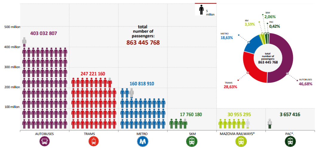
• Annual passenger flow (actual for 2022):
  • The annual passenger flow is approximately 863 million, with buses (403 M) and trams (247 M) handling the majority of passengers. Metro accounts for 161 M passengers, while rail services handle ~53 million combined. The detailed numbers are following:
    • Metro: 160.8 M (18.6% of total volume)
      
    • Trams: 247.2 M (28.6% of total volume)
      
    • Buses: 403 M (46.7% of total volume)
    • Urban Railway (SKM): 17.8 M (2.1% of total volume)
    • Regional Rail (KM within city limits): 31 M (3.6% of total volume)
      
    • Warsaw Commuter Railway (WKD): 3.7 M (0.4% of total volume)-
• Useful details and insights:
  • The network is managed by ZTM (Zarząd Transportu Miejskiego - Public Transport Authority), which handles tickets, schedules and infrastructure.
  • On weekdays, more than 1,500 buses, 400 streetcars, 62 subway trains and 19 units of the Rapid Urban Rail (SKM) are directed to service lines. The transportation network in Warsaw is about 3,600 kilometers, and outside the capital about 1,400 kilometers. In 2022, public transportation carried 863,445,768 passengers.
  • The transportation trends have shifted after COVID-19, but by 2023, passenger numbers returned to pre-pandemic levels with some changed patterns (more weekend travel, slightly different peak hours).
• Recent developments (since 2020):
  • Expanded the M2 metro line to east side
  • Implemented more bus lanes
  • Integrated the system with mobile apps for real-time passengers tracking
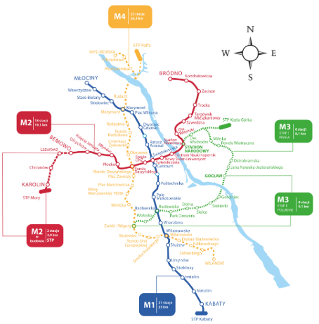
• Development plans:
  • Two new metro lines M3 and M4 are planned.
  • Construction of the M3 line will begin in 2028, no clear date for start of M4 revealed.
  • In 2030, the M3 (shorter route) is expected to carry about 315 thousand passengers per day.
  • According to preliminary assumptions, the M4 line will be 26 km long and have 23 stations, including 2 common for the M4/M2 and M4/M3 lines. There will be several transfer hubs on its route to metro lines M1 (Marymont station), M2 (Rondo Daszyńskiego), M3 (Żwirki i Wigury) and M5 (Plac Narutowicza), as well as to surface public transport and railway lines.

image.png

# downloading the file
url = 'https://mkuran.pl/gtfs/warsaw.zip'
response = requests.get(url)

# creating a ZipFile object from the downloaded content. Originally it is in bytes format, so we convert it in io.BytesIO to simulate a file-like object that zipfile can read from memory
z = zipfile.ZipFile(io.BytesIO(response.content))

# extracting to a directory if it doesn't exist
extract_dir = 'warsaw_gtfs'
os.makedirs(extract_dir, exist_ok=True) # if the directory already exists, an error won't appear
z.extractall(extract_dir)

# displaying the list of extracted files 
files = os.listdir(extract_dir)
print(f'Extracted files: {files}')

Extracted files: ['agency.txt', 'attributions.txt', 'calendar_dates.txt', 'feed_info.txt', 'frequencies.txt', 'routes.txt', 'shapes.txt', 'stops.txt', 'stop_times.txt', 'trips.txt']

🧹 Data Preprocessing

👁️ Initial Data Overview

📐 Enriching Our Analysis Toolkit

Let’s enhance efficiency of our further analysis by creating two functions: get_df_name and data_inspection.

Function: get_df_name

The get_df_name function retrieves and returns the name of a DataFrame variable as a string, what will be handy for displaying information explicitly by other functions.

def get_df_name(df):
    """
    The function returns the user-defined name of the DataFrame variable as a string.

    Input: the DataFrame whose name must be extracted.
    Output: the name of the DataFrame.
    """
    
    for name, value in globals().items():
        if value is df:
            if not name.startswith('_'): # excluding internal names
                return name   
    return "name not found"

Function: data_inspection

The data_inspection function performs comprehensive inspections of a given DataFrame. It provides insights into the dataset’s structure, including concise summaries, examples, descriptive statistics, categorical parameter statistics, missing values, and duplicates.

def data_inspection(df, show_example=True, example_type='head', example_limit=5, frame_len=120):
    """
    The function performs various data inspections on a given DataFrame.
    
    As input it takes:
        - df: a DataFrame to be evaluated.     
        - show_example (bool, optional): whether to display examples of the DataFrame. By default - True.
        - example_type (str, optional): type of examples to display ('sample', 'head', 'tail'). By default - 'head'.
        - example_limit (int, optional): maximum number of examples to display. By default - 5.
        - frame_len (int, optional): the length of frame of printed outputs. Default - 40.
        - frame_len (int, optional): the length of frame of printed outputs. Default - 40. If `show_example` is True, frame_len is set to minimum of the values: manually set `frame_len` and `table_width (which is defined at the project initiation stage).

    As output it presents: 
        - Displays concise summary.
        - Displays examples of the `df` DataFrame (if `show_example` is True)
        - Displays descriptive statistics.
        - Displays descriptive statistics for categorical parameters.
        - Displays information on missing values.
        - Displays information on dublicates.
    """  

    # adjusting output frame; "table_width" is set at project initiation stage
    frame_len = min(table_width, frame_len) if show_example else frame_len
    
    # retrieving a name of the DataFrame
    df_name = get_df_name(df)
    
    # calculating figures on duplicates
    dupl_number = df.duplicated().sum()
    dupl_share = round(df.duplicated().mean()*100, 1)

    # displaying information about the DataFrame
    print('='*frame_len)
    display(Markdown(f'**Overview of `{df_name}`:**'))
    print('-'*frame_len)
    print(f'\033[1mConcise summary:\033[0m')
    print(df.info(), '\n')
    
    if show_example: 
        print('-'*frame_len)
        example_messages = {'sample': 'Random examples', 'head': 'Top rows', 'tail': 'Bottom rows'}
        example_methods = {'sample': df.sample, 'head': df.head, 'tail': df.tail}         
        message = example_messages.get(example_type)       
        method = example_methods.get(example_type)        
        print(f'\033[1m{message}:\033[0m')
        print(method(min(example_limit, len(df))), '\n')      
        
    print('-'*frame_len)
    print(f'\033[1mDescriptive statistics:\033[0m') 
    print(df.describe(), '\n')
    print('-'*frame_len)
    print(f'\033[1mDescriptive statistics of categorical parameters:\033[0m') 
    print(df.describe(include=['object']), '\n')  # printing descriptive statistics for categorical parameters
    
    print('-'*frame_len)
    print(f'\033[1mMissing values:\033[0m') 
    display(df.stb.missing(style=True))
    
    print('-'*frame_len)
    print(f'\033[1mNumber of duplicates\033[0m: {dupl_number} ({dupl_share :.1f}% of all entries)\n')    
    print('='*frame_len)

🔍 Initial Data Examination

# reading the key files and transforming them into DataFrames
stops_df = pd.read_csv(f'{extract_dir}/stops.txt')
routes_df = pd.read_csv(f'{extract_dir}/routes.txt')
trips_df = pd.read_csv(f'{extract_dir}/trips.txt', low_memory=False) # forcing Pandas to read the entire file into memory at once, avoiding DtypeWarnings 
stop_times_df = pd.read_csv(f'{extract_dir}/stop_times.txt', low_memory=False)
frequencies_df = pd.read_csv(f'{extract_dir}/frequencies.txt') 
calendar_dates_df = pd.read_csv(f'{extract_dir}/calendar_dates.txt')

# examination of the main DataFrames 
main_dataframes = [stops_df, routes_df, trips_df, stop_times_df, frequencies_df, calendar_dates_df]

for df in main_dataframes:
    data_inspection(df, show_example=True, example_type='sample', example_limit=5, frame_len=120)

========================================================================================================================

Overview of stops_df:

------------------------------------------------------------------------------------------------------------------------
Concise summary:
<class 'pandas.core.frame.DataFrame'>
RangeIndex: 7096 entries, 0 to 7095
Data columns (total 12 columns):
 #   Column               Non-Null Count  Dtype  
---  ------               --------------  -----  
 0   stop_id              7096 non-null   object 
 1   stop_name            7096 non-null   object 
 2   stop_code            6781 non-null   object 
 3   platform_code        2 non-null      object 
 4   stop_lat             7096 non-null   float64
 5   stop_lon             7096 non-null   float64
 6   location_type        7096 non-null   int64  
 7   parent_station       292 non-null    object 
 8   wheelchair_boarding  7096 non-null   int64  
 9   stop_name_stem       6766 non-null   object 
 10  town_name            6766 non-null   object 
 11  street_name          6702 non-null   object 
dtypes: float64(2), int64(2), object(8)
memory usage: 665.4+ KB
None 

------------------------------------------------------------------------------------------------------------------------
Random examples:
       stop_id                        stop_name stop_code platform_code  \
1355    170501  Kobyłka Żymirskiego-Przychodnia        01           NaN   
4621    402702                     CH Blue City        02           NaN   
5475    503905                          Norblin        05           NaN   
119     102303                         Henryków        03           NaN   
5319  5005M:E3                                3       NaN           NaN   

      stop_lat  stop_lon  location_type parent_station  wheelchair_boarding  \
1355     52.34     21.20              0            NaN                    1   
4621     52.21     20.96              0            NaN                    1   
5475     52.23     20.99              0            NaN                    1   
119      52.33     20.96              0            NaN                    1   
5319     52.23     20.97              2          5005M                    2   

               stop_name_stem town_name       street_name  
1355  Żymirskiego-Przychodnia   Kobyłka  gen. Żymirskiego  
4621            CH  Blue City  Warszawa        Opaczewska  
5475                  Norblin  Warszawa           Żelazna  
119                  Henryków  Warszawa         Mehoffera  
5319                      NaN       NaN               NaN   

------------------------------------------------------------------------------------------------------------------------
Descriptive statistics:
       stop_lat  stop_lon  location_type  wheelchair_boarding
count   7096.00   7096.00        7096.00              7096.00
mean      52.23     21.02           0.08                 1.11
std        0.10      0.12           0.38                 0.31
min       51.92     20.59           0.00                 0.00
25%       52.18     20.95           0.00                 1.00
50%       52.23     21.02           0.00                 1.00
75%       52.28     21.09           0.00                 1.00
max       52.49     21.46           2.00                 2.00 

------------------------------------------------------------------------------------------------------------------------
Descriptive statistics of categorical parameters:
       stop_id stop_name stop_code platform_code parent_station  \
count     7096      7096      6781             2            292   
unique    7096      2884        79             2             38   
top     100101         2        01            M1          1003M   
freq         1        37      2558             1             14   

       stop_name_stem town_name street_name  
count            6766      6766        6702  
unique           2469       321         986  
top           Szkolna  Warszawa  Warszawska  
freq               28      4329         121   

------------------------------------------------------------------------------------------------------------------------
Missing values:

	missing	total	percent
platform_code	7,094	7,096	99.97%
parent_station	6,804	7,096	95.89%
street_name	394	7,096	5.55%
stop_name_stem	330	7,096	4.65%
town_name	330	7,096	4.65%
stop_code	315	7,096	4.44%
stop_id	0	7,096	0.00%
stop_name	0	7,096	0.00%
stop_lat	0	7,096	0.00%
stop_lon	0	7,096	0.00%
location_type	0	7,096	0.00%
wheelchair_boarding	0	7,096	0.00%

------------------------------------------------------------------------------------------------------------------------
Number of duplicates: 0 (0.0% of all entries)

========================================================================================================================
========================================================================================================================

Overview of routes_df:

------------------------------------------------------------------------------------------------------------------------
Concise summary:
<class 'pandas.core.frame.DataFrame'>
RangeIndex: 325 entries, 0 to 324
Data columns (total 7 columns):
 #   Column            Non-Null Count  Dtype 
---  ------            --------------  ----- 
 0   route_id          325 non-null    object
 1   agency_id         325 non-null    int64 
 2   route_short_name  325 non-null    object
 3   route_long_name   325 non-null    object
 4   route_type        325 non-null    int64 
 5   route_color       325 non-null    object
 6   route_text_color  325 non-null    object
dtypes: int64(2), object(5)
memory usage: 17.9+ KB
None 

------------------------------------------------------------------------------------------------------------------------
Random examples:
    route_id  agency_id route_short_name                     route_long_name  \
153      349          0              349  Metro Bemowo – Coopera-Przychodnia   
230      L-3          0              L-3         PKP Piaseczno – Jastrzębiec   
152      340          0              340      Marki Pustelnik – Metro Trocka   
1         10          0               10            Os. Górczewska – Wyścigi   
282      N24          0              N24       PKP Mokry Ług – Dw. Centralny   

     route_type route_color route_text_color  
153           3      880077           FFFFFF  
230           3      000088           FFFFFF  
152           3      880077           FFFFFF  
1             0      B60000           FFFFFF  
282           3      000000           FFFFFF   

------------------------------------------------------------------------------------------------------------------------
Descriptive statistics:
       agency_id  route_type
count     325.00      325.00
mean        0.00        2.72
std         0.00        0.84
min         0.00        0.00
25%         0.00        3.00
50%         0.00        3.00
75%         0.00        3.00
max         0.00        3.00 

------------------------------------------------------------------------------------------------------------------------
Descriptive statistics of categorical parameters:
       route_id route_short_name             route_long_name route_color  \
count       325              325                         325         325   
unique      325              325                         309          12   
top           1                1  Os. Kabaty – Dw. Centralny      880077   
freq          1                1                           4         143   

       route_text_color  
count               325  
unique                2  
top              FFFFFF  
freq                324   

------------------------------------------------------------------------------------------------------------------------
Missing values:

	missing	total	percent
route_id	0	325	0.00%
agency_id	0	325	0.00%
route_short_name	0	325	0.00%
route_long_name	0	325	0.00%
route_type	0	325	0.00%
route_color	0	325	0.00%
route_text_color	0	325	0.00%

------------------------------------------------------------------------------------------------------------------------
Number of duplicates: 0 (0.0% of all entries)

========================================================================================================================
========================================================================================================================

Overview of trips_df:

------------------------------------------------------------------------------------------------------------------------
Concise summary:
<class 'pandas.core.frame.DataFrame'>
RangeIndex: 281950 entries, 0 to 281949
Data columns (total 11 columns):
 #   Column                 Non-Null Count   Dtype  
---  ------                 --------------   -----  
 0   trip_id                281950 non-null  object 
 1   route_id               281950 non-null  object 
 2   service_id             281950 non-null  object 
 3   shape_id               281950 non-null  object 
 4   trip_short_name        2481 non-null    object 
 5   trip_headsign          281950 non-null  object 
 6   direction_id           281950 non-null  int64  
 7   wheelchair_accessible  281950 non-null  int64  
 8   hidden_block_id        281934 non-null  float64
 9   brigade                281934 non-null  object 
 10  fleet_type             281934 non-null  object 
dtypes: float64(1), int64(2), object(8)
memory usage: 23.7+ MB
None 

------------------------------------------------------------------------------------------------------------------------
Random examples:
                          trip_id route_id      service_id           shape_id  \
278533    2025-04-18:9:PtS:3:1345        9  2025-04-18:PtS  2025-04-18:148466   
168703  2025-04-15:326:PcS:4:1153      326  2025-04-15:PcS  2025-04-15:141491   
51720   2025-04-11:218:PtS:1:0659      218  2025-04-11:PtS  2025-04-11:145583   
62426    2025-04-11:71:PtS:2:1322       71  2025-04-11:PtS  2025-04-11:153875   
160385  2025-04-15:188:PcS:3:2114      188  2025-04-15:PcS  2025-04-15:141542   

       trip_short_name      trip_headsign  direction_id  \
278533             NaN  P+R Al. Krakowska             0   
168703             NaN       Metro Bródno             0   
51720              NaN     Metro Wierzbno             1   
62426              NaN      PKP Służewiec             0   
160385             NaN       PKP Gocławek             0   

        wheelchair_accessible  hidden_block_id brigade fleet_type  
278533                      1        313513.00       3       120N  
168703                      1        295476.00       4    M-np12m  
51720                       1        306394.00       1    G-np18m  
62426                       1        329793.00       2       120N  
160385                      1        295981.00       3    G-np18m   

------------------------------------------------------------------------------------------------------------------------
Descriptive statistics:
       direction_id  wheelchair_accessible  hidden_block_id
count     281950.00              281950.00        281934.00
mean           0.50                   1.04        305577.97
std            0.50                   0.20         42510.68
min            0.00                   1.00        100736.00
25%            0.00                   1.00        294592.00
50%            1.00                   1.00        313850.00
75%            1.00                   1.00        336156.00
max            1.00                   2.00        350142.00 

------------------------------------------------------------------------------------------------------------------------
Descriptive statistics of categorical parameters:
                           trip_id route_id      service_id  \
count                       281950   281950          281950   
unique                      281950      325              13   
top     2025-04-10:102:PcS:09:1426        2  2025-04-11:PtS   
freq                             1     4165           34129   

                 shape_id trip_short_name  trip_headsign brigade fleet_type  
count              281950            2481         281950  281934     281934  
unique              13835             322            365     451         16  
top     2025-04-10:157566         99280/1  Metro Młociny       1    G-np18m  
freq                  206               9          10306   41408     104644   

------------------------------------------------------------------------------------------------------------------------
Missing values:

	missing	total	percent
trip_short_name	279,469	281,950	99.12%
hidden_block_id	16	281,950	0.01%
brigade	16	281,950	0.01%
fleet_type	16	281,950	0.01%
trip_id	0	281,950	0.00%
route_id	0	281,950	0.00%
service_id	0	281,950	0.00%
shape_id	0	281,950	0.00%
trip_headsign	0	281,950	0.00%
direction_id	0	281,950	0.00%
wheelchair_accessible	0	281,950	0.00%

------------------------------------------------------------------------------------------------------------------------
Number of duplicates: 0 (0.0% of all entries)

========================================================================================================================
========================================================================================================================

Overview of stop_times_df:

------------------------------------------------------------------------------------------------------------------------
Concise summary:
<class 'pandas.core.frame.DataFrame'>
RangeIndex: 7706414 entries, 0 to 7706413
Data columns (total 7 columns):
 #   Column          Dtype 
---  ------          ----- 
 0   trip_id         object
 1   stop_sequence   int64 
 2   stop_id         object
 3   arrival_time    object
 4   departure_time  object
 5   pickup_type     int64 
 6   drop_off_type   int64 
dtypes: int64(3), object(4)
memory usage: 411.6+ MB
None 

------------------------------------------------------------------------------------------------------------------------
Random examples:
                             trip_id  stop_sequence stop_id arrival_time  \
5606476   2025-04-16:414:PcS:06:1725             23  108302     18:12:00   
2705836    2025-04-13:173:NdS:5:1416              3  211802     14:19:00   
822128     2025-04-10:78:PcS:08:1734             13  506305     17:58:00   
4955651  2025-04-16:102:PcS:542:0848              8  211802     09:00:00   
5873426    2025-04-16:S1:PcS:17:1500             23    4905     16:07:00   

        departure_time  pickup_type  drop_off_type  
5606476       18:12:00            0              0  
2705836       14:19:00            0              0  
822128        17:58:00            0              0  
4955651       09:00:00            0              0  
5873426       16:07:00            0              0   

------------------------------------------------------------------------------------------------------------------------
Descriptive statistics:
       stop_sequence  pickup_type  drop_off_type
count     7706414.00   7706414.00     7706414.00
mean           15.66         0.77           0.77
std            11.24         1.31           1.31
min             0.00         0.00           0.00
25%             7.00         0.00           0.00
50%            14.00         0.00           0.00
75%            23.00         3.00           3.00
max            74.00         3.00           3.00 

------------------------------------------------------------------------------------------------------------------------
Descriptive statistics of categorical parameters:
                          trip_id  stop_id arrival_time departure_time
count                     7706414  7706414      7706414        7706414
unique                     281950     6805         1611           1611
top     2025-04-15:N02:PcS:3:2652   701306     07:20:00       07:20:00
freq                           75     8457         8506           8495 

------------------------------------------------------------------------------------------------------------------------
Missing values:

	missing	total	percent
trip_id	0	7,706,414	0.00%
stop_sequence	0	7,706,414	0.00%
stop_id	0	7,706,414	0.00%
arrival_time	0	7,706,414	0.00%
departure_time	0	7,706,414	0.00%
pickup_type	0	7,706,414	0.00%
drop_off_type	0	7,706,414	0.00%

------------------------------------------------------------------------------------------------------------------------
Number of duplicates: 0 (0.0% of all entries)

========================================================================================================================
========================================================================================================================

Overview of frequencies_df:

------------------------------------------------------------------------------------------------------------------------
Concise summary:
<class 'pandas.core.frame.DataFrame'>
RangeIndex: 101 entries, 0 to 100
Data columns (total 5 columns):
 #   Column        Non-Null Count  Dtype 
---  ------        --------------  ----- 
 0   trip_id       101 non-null    object
 1   start_time    101 non-null    object
 2   end_time      101 non-null    object
 3   headway_secs  101 non-null    int64 
 4   exact_times   101 non-null    int64 
dtypes: int64(2), object(3)
memory usage: 4.1+ KB
None 

------------------------------------------------------------------------------------------------------------------------
Random examples:
       trip_id start_time  end_time  headway_secs  exact_times
44  M1:SbM:KAB   20:37:00  22:50:00           450            0
43  M1:SbM:KAB   07:23:00  20:37:00           300            0
13  M1:PcM:KAB   21:03:00  22:21:00           390            0
10  M1:PcM:KAB   09:23:00  13:55:00           210            0
66  M2:PcM:BRO   05:59:00  06:22:00           270            0 

------------------------------------------------------------------------------------------------------------------------
Descriptive statistics:
       headway_secs  exact_times
count        101.00       101.00
mean         397.43         0.08
std          194.30         0.27
min          150.00         0.00
25%          270.00         0.00
50%          390.00         0.00
75%          480.00         0.00
max          900.00         1.00 

------------------------------------------------------------------------------------------------------------------------
Descriptive statistics of categorical parameters:
           trip_id start_time  end_time
count          101        101       101
unique          16         60        68
top     M1:PtM:KAB   05:00:00  26:08:59
freq             9         16         2 

------------------------------------------------------------------------------------------------------------------------
Missing values:

	missing	total	percent
trip_id	0	101	0.00%
start_time	0	101	0.00%
end_time	0	101	0.00%
headway_secs	0	101	0.00%
exact_times	0	101	0.00%

------------------------------------------------------------------------------------------------------------------------
Number of duplicates: 0 (0.0% of all entries)

========================================================================================================================
========================================================================================================================

Overview of calendar_dates_df:

------------------------------------------------------------------------------------------------------------------------
Concise summary:
<class 'pandas.core.frame.DataFrame'>
RangeIndex: 62 entries, 0 to 61
Data columns (total 3 columns):
 #   Column          Non-Null Count  Dtype 
---  ------          --------------  ----- 
 0   date            62 non-null     int64 
 1   service_id      62 non-null     object
 2   exception_type  62 non-null     int64 
dtypes: int64(2), object(1)
memory usage: 1.6+ KB
None 

------------------------------------------------------------------------------------------------------------------------
Random examples:
        date      service_id  exception_type
54  20250418             PtM               1
38  20250410             PcM               1
15  20250505  2025-04-14:PcS               1
36  20250503             NdM               1
17  20250422  2025-04-15:PcS               1 

------------------------------------------------------------------------------------------------------------------------
Descriptive statistics:
             date  exception_type
count       62.00           62.00
mean  20250447.58            1.00
std         40.64            0.00
min   20250410.00            1.00
25%   20250417.25            1.00
50%   20250425.00            1.00
75%   20250502.75            1.00
max   20250510.00            1.00 

------------------------------------------------------------------------------------------------------------------------
Descriptive statistics of categorical parameters:
       service_id
count          62
unique         13
top           PcM
freq           15 

------------------------------------------------------------------------------------------------------------------------
Missing values:

	missing	total	percent
date	0	62	0.00%
service_id	0	62	0.00%
exception_type	0	62	0.00%

------------------------------------------------------------------------------------------------------------------------
Number of duplicates: 0 (0.0% of all entries)

========================================================================================================================

# checking unique values and their count of each main DataFrame and each column 
for df in main_dataframes:
    display(Markdown(f'**`{get_df_name(df)}`**'))
    for parameter in df.columns:
        print('='*100)
        print(f'\033[1m`{parameter}`\033[0m')
        df[parameter].value_counts()
    print()    

stops_df

====================================================================================================
`stop_id`

stop_id
100101    1
406701    1
407101    1
407004    1
407002    1
         ..
221002    1
221001    1
220904    1
220902    1
7903      1
Name: count, Length: 7096, dtype: int64

====================================================================================================
`stop_name`

stop_name
2                       37
1                       37
3                       33
4                       31
5                       28
                        ..
Młochów Leśniczówka      1
Krakowiany               1
Wola Krakowiańska        1
Jastrzębiec Garbatka     1
Warszawa Gdańska         1
Name: count, Length: 2884, dtype: int64

====================================================================================================
`stop_code`

stop_code
01     2558
02     2413
03      538
04      494
05      171
       ... 
76        1
C12       1
19        1
57        1
20        1
Name: count, Length: 79, dtype: int64

====================================================================================================
`platform_code`

platform_code
M1    1
M2    1
Name: count, dtype: int64

====================================================================================================
`stop_lat`

stop_lat
52.25    3
52.36    2
52.20    2
52.20    2
52.25    2
        ..
52.18    1
52.19    1
52.19    1
52.19    1
52.26    1
Name: count, Length: 7002, dtype: int64

====================================================================================================
`stop_lon`

stop_lon
21.04    2
20.93    2
21.15    2
21.00    2
20.90    2
        ..
21.15    1
21.15    1
21.14    1
21.14    1
20.99    1
Name: count, Length: 7027, dtype: int64

====================================================================================================
`location_type`

location_type
0    6805
2     253
1      38
Name: count, dtype: int64

====================================================================================================
`parent_station`

parent_station
1003M    14
3228M    13
7088M    12
7019M    11
7014M    11
3114M    11
6005M    10
5034M    10
5030M    10
3281M     9
7013M     9
5005M     9
3282M     9
7099M     9
3230M     9
5028M     8
6003M     8
3132M     8
1231M     8
3009M     8
7006M     8
5040M     8
1146M     7
3280M     7
3279M     7
1085M     7
5032M     6
7043M     6
1526M     5
3127M     5
1140M     5
1411M     4
7079M     4
1137M     4
6006M     4
6052M     3
6055M     3
6059M     3
Name: count, dtype: int64

====================================================================================================
`wheelchair_boarding`

wheelchair_boarding
1    6344
2     751
0       1
Name: count, dtype: int64

====================================================================================================
`stop_name_stem`

stop_name_stem
Szkolna             28
Polna               23
Cmentarz            22
Metro Młociny       20
Wiatraczna          18
                    ..
Kołłątaja            1
Kupiecka             1
Zieleniecka          1
Szamoty              1
Warszawa Gdańska     1
Name: count, Length: 2469, dtype: int64

====================================================================================================
`town_name`

town_name
Warszawa               4329
Legionowo                92
Konstancin-Jeziorna      92
Piaseczno                87
Otwock                   73
                       ... 
Głosków-Letnisko          1
Kosów                     1
Hornówek                  1
Sieraków                  1
Brzeziny                  1
Name: count, Length: 321, dtype: int64

====================================================================================================
`street_name`

street_name
Warszawska           121
Puławska              86
al. Krakowska         77
Modlińska             73
Al. Jerozolimskie     63
                    ... 
Bema                   1
Cegielniana            1
Korotyńskiego          1
Olsztyńska             1
Bielańska              1
Name: count, Length: 986, dtype: int64

routes_df

====================================================================================================
`route_id`

route_id
1      1
729    1
817    1
815    1
809    1
      ..
207    1
204    1
203    1
202    1
Z33    1
Name: count, Length: 325, dtype: int64

====================================================================================================
`agency_id`

agency_id
0    325
Name: count, dtype: int64

====================================================================================================
`route_short_name`

route_short_name
1      1
729    1
817    1
815    1
809    1
      ..
207    1
204    1
203    1
202    1
Z33    1
Name: count, Length: 325, dtype: int64

====================================================================================================
`route_long_name`

route_long_name
Os. Kabaty – Dw. Centralny               4
Cm. Północny-Brama Gł. – Pl. Wilsona     2
Os. Górczewska – Dw. Centralny           2
Chomiczówka – Wilanów                    2
Dziekanów Leśny – Metro Młociny          2
                                        ..
Fort Wawrzyszew – Metro Młociny          1
PKP Gocławek – Metro Stadion Narodowy    1
Metro Księcia Janusza – Nowe Bemowo      1
Żerań FSO – Boernerowo                   1
Rondo „Radosława” – Włościańska          1
Name: count, Length: 309, dtype: int64

====================================================================================================
`route_type`

route_type
3    291
0     27
2      5
1      2
Name: count, dtype: int64

====================================================================================================
`route_color`

route_color
880077    143
B60000     52
000088     42
000000     42
006800     39
0000BB      1
BB0000      1
E84A4B      1
2E8EC8      1
FFAC01      1
2F7B20      1
70AD46      1
Name: count, dtype: int64

====================================================================================================
`route_text_color`

route_text_color
FFFFFF    324
000000      1
Name: count, dtype: int64

trips_df

====================================================================================================
`trip_id`

trip_id
2025-04-10:102:PcS:09:1426    1
2025-04-16:14:PcS:2:2023      1
2025-04-16:14:PcS:3:0651      1
2025-04-16:14:PcS:3:0604      1
2025-04-16:14:PcS:3:0517      1
                             ..
2025-04-13:133:NdS:2:0835     1
2025-04-13:133:NdS:2:0852     1
2025-04-13:133:NdS:2:0915     1
2025-04-13:133:NdS:2:0932     1
M2:SbM:BRO                    1
Name: count, Length: 281950, dtype: int64

====================================================================================================
`route_id`

route_id
2      4165
16     4025
9      3922
1      3826
33     3476
       ... 
320      45
800      24
N58      15
M1        8
M2        8
Name: count, Length: 325, dtype: int64

====================================================================================================
`service_id`

service_id
2025-04-11:PtS    34129
2025-04-10:PcS    34116
2025-04-14:PcS    34116
2025-04-15:PcS    34116
2025-04-16:PcS    34116
2025-04-17:PcS    33349
2025-04-18:PtS    33266
2025-04-12:SbS    22393
2025-04-13:NdS    22333
NdM                   4
PcM                   4
PtM                   4
SbM                   4
Name: count, dtype: int64

====================================================================================================
`shape_id`

shape_id
2025-04-10:157566    206
2025-04-17:157566    206
2025-04-14:157566    206
2025-04-15:157566    206
2025-04-11:157566    206
                    ... 
2025-04-17:145751      1
2025-04-12:123372      1
2025-04-12:123383      1
2025-04-12:123381      1
2025-04-12:161936      1
Name: count, Length: 13835, dtype: int64

====================================================================================================
`trip_short_name`

trip_short_name
99280/1    9
99302/3    9
10810/1    9
97212/3    9
10820/1    9
          ..
99460/1    2
11262/3    2
99468/9    2
99481      2
11284/5    2
Name: count, Length: 322, dtype: int64

====================================================================================================
`trip_headsign`

trip_headsign
Metro Młociny        10306
P+R Al. Krakowska     7712
Dw. Centralny         7047
Metro Wilanowska      6637
Os. Górczewska        6303
                     ...  
Kabaty                   4
Młociny                  4
Bemowo                   4
Bródno                   4
PKP Rembertów            2
Name: count, Length: 365, dtype: int64

====================================================================================================
`direction_id`

direction_id
1    141316
0    140634
Name: count, dtype: int64

====================================================================================================
`wheelchair_accessible`

wheelchair_accessible
1    270141
2     11809
Name: count, dtype: int64

====================================================================================================
`hidden_block_id`

hidden_block_id
329692.00    315
269155.00    300
269157.00    295
138107.00    290
339368.00    285
            ... 
336802.00      1
336531.00      1
329854.00      1
310162.00      1
306225.00      1
Name: count, Length: 7671, dtype: int64

====================================================================================================
`brigade`

brigade
1      41408
2      36290
3      28899
4      22261
5      17858
       ...  
745       15
754       14
M11       12
M10       12
777       12
Name: count, Length: 451, dtype: int64

====================================================================================================
`fleet_type`

fleet_type
G-np18m      104644
M-np12m       68739
K-np8-10m     28880
120N          22156
DUO           16177
H-el18m       13707
2 wagony      11809
116N/142N      5450
L-el12m        4373
134N           3518
27WE           1069
2x45WEa         546
35WEa           470
2x31WEba        238
45WEa            80
31WEba           78
Name: count, dtype: int64

stop_times_df

====================================================================================================
`trip_id`

trip_id
2025-04-15:N02:PcS:3:2652      75
2025-04-12:N02:SbS:4:2420      75
2025-04-17:N02:PcS:3:2652      75
2025-04-10:N02:PcS:297:2752    75
2025-04-14:N02:PcS:4:2722      75
                               ..
2025-04-15:7:PcS:08:1436        2
2025-04-15:7:PcS:08:0434        2
2025-04-18:517:PtS:8:0800       2
2025-04-18:517:PtS:8:0631       2
2025-04-10:320:PcS:787:0804     2
Name: count, Length: 281950, dtype: int64

====================================================================================================
`stop_sequence`

stop_sequence
1     281950
2     281790
3     281546
4     281315
5     278401
       ...  
70       306
71       162
72       117
73        72
74        36
Name: count, Length: 75, dtype: int64

====================================================================================================
`stop_id`

stop_id
701306    8457
404401    8297
707102    7926
703706    7926
700902    7926
          ... 
617602       7
617802       7
617902       7
617702       7
286102       4
Name: count, Length: 6805, dtype: int64

====================================================================================================
`arrival_time`

arrival_time
07:20:00    8506
16:04:00    8473
07:28:00    8471
07:30:00    8467
16:44:00    8437
            ... 
00:16:00       4
00:30:00       4
00:26:00       4
00:07:00       4
00:11:00       4
Name: count, Length: 1611, dtype: int64

====================================================================================================
`departure_time`

departure_time
07:20:00    8495
07:28:00    8480
16:04:00    8464
07:30:00    8458
16:44:00    8453
            ... 
00:14:00       4
00:32:00       4
00:30:00       4
00:26:00       4
00:11:00       4
Name: count, Length: 1611, dtype: int64

====================================================================================================
`pickup_type`

pickup_type
0    5729570
3    1976844
Name: count, dtype: int64

====================================================================================================
`drop_off_type`

drop_off_type
0    5729570
3    1976844
Name: count, dtype: int64

frequencies_df

====================================================================================================
`trip_id`

trip_id
M1:PtM:KAB    9
M1:PtM:MLO    9
M2:PtM:BEM    9
M2:PtM:BRO    9
M1:PcM:KAB    8
M1:PcM:MLO    8
M2:PcM:BRO    8
M2:PcM:BEM    7
M1:SbM:KAB    5
M1:SbM:MLO    5
M2:SbM:BEM    5
M2:SbM:BRO    5
M1:NdM:KAB    4
M1:NdM:MLO    4
M2:NdM:BEM    3
M2:NdM:BRO    3
Name: count, dtype: int64

====================================================================================================
`start_time`

start_time
05:00:00    16
24:12:00     2
20:54:00     2
24:08:00     2
19:01:00     2
24:18:00     2
14:21:00     2
22:50:00     2
09:20:00     2
13:25:00     2
20:37:00     2
06:22:00     2
05:59:00     2
19:30:00     2
14:24:00     2
09:32:00     2
05:31:00     2
06:59:00     2
08:46:00     2
24:13:00     2
23:37:00     2
05:50:00     2
09:23:00     2
05:48:00     2
13:55:00     2
22:44:00     2
05:33:00     2
23:15:00     1
06:49:00     1
20:10:00     1
22:51:00     1
19:31:00     1
20:42:00     1
20:32:00     1
06:08:00     1
21:33:00     1
20:00:00     1
06:39:00     1
22:32:00     1
08:29:00     1
09:17:00     1
21:12:00     1
08:33:00     1
20:28:00     1
20:02:00     1
21:03:00     1
22:21:00     1
19:20:00     1
22:09:00     1
19:59:00     1
21:09:00     1
21:37:00     1
19:17:00     1
07:23:00     1
05:23:00     1
19:53:00     1
23:01:00     1
09:22:00     1
22:36:00     1
23:39:00     1
Name: count, dtype: int64

====================================================================================================
`end_time`

end_time
26:08:59    2
20:54:00    2
24:08:00    2
24:18:00    2
26:18:59    2
           ..
19:53:00    1
23:01:00    1
09:22:00    1
22:36:00    1
23:39:00    1
Name: count, Length: 68, dtype: int64

====================================================================================================
`headway_secs`

headway_secs
270    12
390    12
480     9
450     8
150     8
900     8
180     8
570     7
210     6
300     6
420     5
540     5
360     4
330     2
510     1
Name: count, dtype: int64

====================================================================================================
`exact_times`

exact_times
0    93
1     8
Name: count, dtype: int64

calendar_dates_df

====================================================================================================
`date`

date
20250410    2
20250415    2
20250502    2
20250425    2
20250418    2
20250508    2
20250424    2
20250417    2
20250507    2
20250430    2
20250423    2
20250416    2
20250506    2
20250429    2
20250422    2
20250505    2
20250411    2
20250428    2
20250414    2
20250504    2
20250503    2
20250501    2
20250427    2
20250421    2
20250420    2
20250413    2
20250510    2
20250426    2
20250419    2
20250412    2
20250509    2
Name: count, dtype: int64

====================================================================================================
`service_id`

service_id
PcM               15
2025-04-13:NdS     7
NdM                7
PtM                5
2025-04-12:SbS     4
2025-04-15:PcS     4
2025-04-16:PcS     4
2025-04-18:PtS     4
SbM                4
2025-04-14:PcS     3
2025-04-17:PcS     3
2025-04-10:PcS     1
2025-04-11:PtS     1
Name: count, dtype: int64

====================================================================================================
`exception_type`

exception_type
1    62
Name: count, dtype: int64

Consistent match between stop_id and stop_name (lack of cases where one stop_id value has multiple stop_name values or vice versa) is crucial for our study. Let’s examine it these connections.

# checking that each `stop_id` has only one unique `stop_name` and vice versa
print(f'\033[1mChecking number of stop names for each stop id\033[0m (data is sorted):')
stops_df.groupby('stop_id')['stop_name'].value_counts().sort_values()

print(f'\n\033[1mChecking number of stop ids for each stop name\033[0m (data is sorted):')
stops_df.groupby('stop_name')['stop_id'].value_counts().sort_values()

Checking number of stop names for each stop id (data is sorted):

stop_id  stop_name       
100101   Kijowska            1
407004   Łazy                1
407002   Łazy                1
407001   Łazy                1
406902   Łazy Podleśna       1
                            ..
220904   Bronowska           1
220902   Bronowska           1
220901   Bronowska           1
221302   Cyklamenów          1
7903     Warszawa Gdańska    1
Name: count, Length: 7096, dtype: int64

Checking number of stop ids for each stop name (data is sorted):

stop_name                     stop_id 
1                             1003M:E1    1
Polfa                         110201      1
Poleczki                      301304      1
                              301303      1
                              301302      1
                                         ..
Konstancin-Jeziorna Cmentarz  386202      1
                              386201      1
Konstancin-Jeziorna Chopina   310102      1
Konstancin-Jeziorna Jasna     317602      1
Żółkiewskiego                 201204      1
Name: count, Length: 7096, dtype: int64

# checking `stop_id` values presence
print(f'\033[1mUnique `stop_id` values:\033[0m')
print(' - `stops_df`:', stops_df['stop_id'].nunique())
print(' - `stop_times_df`:', stop_times_df['stop_id'].nunique())

common_stop_ids = set(stops_df['stop_id']).intersection(stop_times_df['stop_id'])
print(f"\n\033[1mNumber of common `stop_id` values in `stops_df' and `stop_times_df` :\033[0m {len(common_stop_ids)}")

stop_times_stops_list = stop_times_df['stop_id'].unique()
excluded_stops = stops_df.query('stop_id not in @stop_times_stops_list')

print(f'\n\033[1mExcluded stops:\033[0m {len(excluded_stops["stop_id"])} ({len(excluded_stops["stop_id"]) / stops_df["stop_id"].nunique() :0.1%} of total)')

print('\n\033[1mSample of excluded stops:\033[0m')
print(excluded_stops.sample(3, random_state=7))

Unique `stop_id` values:
 - `stops_df`: 7096
 - `stop_times_df`: 6805

Number of common `stop_id` values in `stops_df' and `stop_times_df` : 6805

Excluded stops: 291 (4.1% of total)

Sample of excluded stops:
       stop_id         stop_name stop_code platform_code  stop_lat  stop_lon  \
5450  5034M:E7                 7       NaN           NaN     52.24     20.91   
673      1231M  Stadion Narodowy       C14           NaN     52.25     21.04   
3322  3127M:E1                 1       NaN           NaN     52.16     21.03   

      location_type parent_station  wheelchair_boarding stop_name_stem  \
5450              2          5034M                    1            NaN   
673               1            NaN                    1            NaN   
3322              2          3127M                    1            NaN   

     town_name street_name  
5450       NaN         NaN  
673        NaN         NaN  
3322       NaN         NaN  

Observations

• stops_df (stops.txt)

  • 7,107 stops, as expected, most concentrated in Warszawa (4,343 stops), while some neighborhoods are also covered, e.g. Legionowo (92 stops)
  • Platform codes (99.97%) and parent stations (95.89%) mostly missing.
  • street_name, stop_name_stem, town_name, stop_code consist about 5% of missing values.
  • Geospatial data (latitude, longitude) is available, no missing values.
  • No duplicates revealed
  • The distribution of location_type values indicates that:
    • Warsaw’s public transport network consists of a large number of individual stops/platforms - 6816 (location_type = 0), that serve as the primary boarding and alighting locations for passengers.
    • There are 38 major stations (unique stop_id values) that act as larger transit hubs (location_type = 1), possibly containing multiple platforms or stops within them.
    • There are 253 entrances or exits (location_type = 253) for larger transit stations (e.g., metro entrances).

  💡💡 The revealed 38 transit hubs are likely the best areas (in terms of people traffic) for launching new pizzerias.

  Note: According to the GTFS Specification, stops with location_type = 1 do not have specific arrival or departure times. Instead, these times are assigned to the individual stops or platforms (with location_type = 0) that are part of the station. So we won’t see stop_id values associated with location_type = 1 in the stop_times_df DataFrame.

---

• routes_df (routes.txt)
  • Warsaw’s public transport system has 325 routes in total, where:
    • bus routes - 290 (route_type = 3)
    • tram/light rail routes - 28 (route_type = 0)
    • rail routes - 5 (route_type = 2)
    • metro lines - 2 (route_type = 1)
  • No missing values or duplicates revealed
  💡 Buses are the majority of Warsaw’s transport network.
  💡 Route data is well-structured for analysis.

---

• trips_df (trips.txt)
  • 280,090 trips in total
  • Most common destination: “Metro Młociny”`.
  • "trip_short_name" is 99.11% missing.
  • The other columns have no missing values or a very minor number (16 - 0.01% of total)
  • There are extremely popular routes that appear in the dataset 3-4k times (e.g.route_id 2, 9, 1), meanwhile there routes with suspiciously low number of entries, e.g. for metro, where routes M1 and M2 have just 8 appearances each.
  • Vehical types are available (fleet_type) for each trip. Thus we may try to retrieve approximate passenger capacity in case we need more precise estimations for future comparison of each trip and route impact.
  💡️ Trip short names are unreliable.
  💡 A high number of trips is available for reliable conclusions.
  💡💡 Data on metro trips seems to be insufficient. A GTFS feed should ideally list every stop time for every trip. A metro, tends to operate very frequently, thus the low count of just 8 entries suggests a potential issue with the data.

---

• stop_times_df (stop_times.txt)
  • 7,700,837 records.
  • Top travel time: "07:30:00" (morning rush hour).
  • Most stops have standard pickup dropoff types. However, about 25% of stops have a special drop-off type (drop_off_type = 3), which means passengers must coordinate with the driver to be picked up or dropped off. These stops may experience lower traffic compared to regular stops, as they require extra effort from passengers and may not be as frequently used. We may take this into account to downscale the impact of such stops if we need more precise estimations for future stops comparisons.
  • No missing values or duplicates revealed
  💡 Highly detailed transport schedules available.
  💡 We see a strong morning rush-hour traffic.
  💡💡 About 25% of stops may generate less traffic compared to regular stops.

---

• frequencies_df (frequencies.txt)
  • 101 records (most routes use fixed schedules).
  • Applied to metro only as likely it only uses frequency-based scheduling.
  • Average wait time is 6.5 min.
  • Shortest wait time is 2.5 min (peak time), longest wait time is 15 min.
  • No missing values or duplicates revealed
  💡 Headway data is available only for the metro, with wait times ranging from 2.5 to 15 minutes.

---

• calendar_dates_df (calendar_dates.txt)
  • 62 records, all of them with exception_type = 1, which indicates that service is available on these days dates.
  • The scheduled period covers two months: 18 March 2025 - 17 April 2025.
    
  • No missing values or duplicates revealed

---

• Overall conclusions
  • Data quality and integrity
    • Despite non-optimal data types and some missing values in non-critical columns (all the key columns relevant to our study are complete), the data is sufficient for further analysis and addressing these minor issues would not significantly impact the results.
    • No duplicates revealed among all the entries of all the DataFrames.
    • We proved consistent match between stop_id and stop_name (lack of cases where one stop_id value has multiple stop_name values or vice versa).
    • There are 291 stop_id values of stops_df (4.1% of total) not included in stop_times_df and thus they won’t appear in further analysis.
      • These excluded stops may represent for instance stops that are not currently in use, planned future stops, parent stations (location_type = 1) that don’t have specific arrival or departure times.
    • The DataFrames are interconnected - they have columns in common. In the next step we will describe these connections, what will be helpful for further study.
    • 💡 There is no calendar.txt file in the GTFS feed, what means that all service availability is defined in calendar_dates.txt instead.
      
    • ⚠ The two month period (18 March 2025 to 17 April 2025) is sufficient for the purpose of our study. While seasonal fluctuations are not covered, this is not a critical issue since our focus is on comparing traffic at different transport hubs rather than analyzing trends in passenger flows over time. Therefore, this dataset can be considered reliable for our analysis.
  • Business implications
    • Bus is a leading transport.
    • Data allows mapping busiest hubs, in particular all the geospatial data is available.
    • We revealed the rush-hour peak ~07:30 AM.
    • We revealed that about 25% of stops may experience lower traffic compared to regular stops (due to the additional effort required for passenger pick-up or drop-off). We have chosen to simplify the study and ignore this feature for the time being.
    • Vehicle type data allows future comparison of trip and route impact based on passenger loading, these data must be investigated futher.
    • ⚠ The main concern is the lack of metro trip data. Metro passengers account for about 19% of total passenger flow, meaning we can still proceed with the analysis. However, due to incomplete metro trip data, we will need additional sources to address this part of the study.

---

🔗 Main Files Relationships

Let’s describe the relationships among the main tables, as it will be helpful for further analysis.
While we could create a full relationship diagram of all the tables, for now, describing the key columns and their connections will be sufficient.

Main files relationships

File	Key columns	Connected file
stops.txt	stop_id	stop_times.txt
routes.txt	route_id	trips.txt
trips.txt	trip_id, route_id	stop_times.txt(via trip_id), frequencies.txt(via trip_id)*, routes.txt (via route_id)
stop_times.txt	trip_id, stop_id	stops.txt (via stop_id), frequencies.txt(via trip_id)*, trips.txt (via trip_id)
frequencies.txt	trip_id	trips.txt, stop_times.txt
calendar_dates.txt	service_id	trips.txt

*Note: In GTFS, the same trip_id is used with different meanings across the files. Where in trips.txt and stop_times.txt, trip_id represents a specific trip with exact arrival/departure times at each stop. While in frequencies.txt, the same trip_id is used to indicate regular intervals (headways) during specified time periods.

🛠️ Addressing Data Issues

Let’s check the trip_id column of stop_times_df Dataframe. That will be an extra check of the metro trips data.

# filtering M1 and M2 metro routes
metro_stop_times = stop_times_df[stop_times_df['trip_id'].str.contains('M1|M2')]

print(f'Number of metro stop times: {len(metro_stop_times)}')
print(metro_stop_times.head())

Number of metro stop times: 15507
                           trip_id  stop_sequence stop_id arrival_time  \
51556  2025-04-10:114:PcS:M22:0749              0  605920     07:49:00   
51557  2025-04-10:114:PcS:M22:0749              1  605903     07:51:00   
51558  2025-04-10:114:PcS:M22:0749              2  606101     07:52:00   
51559  2025-04-10:114:PcS:M22:0749              3  601502     07:54:00   
51560  2025-04-10:114:PcS:M22:0749              4  601602     07:55:00   

      departure_time  pickup_type  drop_off_type  
51556       07:49:00            0              0  
51557       07:51:00            0              0  
51558       07:52:00            3              3  
51559       07:54:00            3              3  
51560       07:55:00            0              0  

The result number of metro stop times is 14388. It means, that the trip_id contains M1 and M2, but it also contains unsuitable data like “2025-03-18:114:PcS:M22:0749”. So the string can contain “M2” but it’s not our metro.

The calendar_dates_df must have a common key with metro, while the stops_df file must have thetrip_ids. We can filter the trip_id using the known values from the routes_df.

# filtering routes for metro (route_type == 1)
metro_routes = routes_df[routes_df['route_type'] == 1]
metro_route_ids = metro_routes['route_id'].tolist()
metro_trips = trips_df[trips_df['route_id'].isin(metro_route_ids)]

# getting the `trip_ids` for metro trips
metro_trip_ids = metro_trips['trip_id'].tolist()

# filtering the `stop_times_df`for metro the `trip_ids`
metro_stop_times_v2 = stop_times_df[stop_times_df['trip_id'].isin(metro_trip_ids)]

print(f'\033[1mNumber of metro stop times:\033[0m {len(metro_stop_times_v2)}')
print(metro_stop_times_v2.head())

Number of metro stop times: 312
            trip_id  stop_sequence   stop_id arrival_time departure_time  \
7706102  M1:NdM:KAB              0  6059M:P1     00:00:00       00:00:00   
7706103  M1:NdM:KAB              1  6055M:P1     00:02:00       00:02:00   
7706104  M1:NdM:KAB              2  6052M:P1     00:04:00       00:04:00   
7706105  M1:NdM:KAB              3  6006M:P1     00:06:00       00:06:00   
7706106  M1:NdM:KAB              4  6005M:P1     00:07:00       00:07:00   

         pickup_type  drop_off_type  
7706102            0              0  
7706103            0              0  
7706104            0              0  
7706105            0              0  
7706106            0              0  

The latest results, showing 312 metro stop times are already more reasonable than before, but still look very strange. There are routes that appear in the dataset thousands times while having less frequent stops (e.g., comparing railway and metro). However, it must be correct data, that describes this particular GTFS dataset.

📊 Exploratory Data Analysis (EDA)

✨ Enriching the Data

⚠ Since our priority is to identify busy non-central stops, we will flag stops that are far from the city center. For this purpose we will set Warsaw Central Station (Warszawa Centralna) as the central point (its location is in the very busy central part of the city close to many business centers and popular places of interest like Palace of Culture and Science) and we will define the central part of the city as the area within 4 km of it.

It’s easy to find Warsaw Central Station coordinates on the map (they are following: 52.2319, 21.0067). To calculate the distance between a stop and the city center we will utilize the “geopy.distance” module of the from the “geopy” library. We will create additional columns in the stops_df DataFrame, indicating whether a stop is considered as a central or not.

# creating new columns describing whether a station is central
city_center = (52.2319, 21.0067)  # latitude and longitude of Warsaw Central Station 

stops_df['distance_to_center'] = stops_df.apply(lambda row: geodesic((row['stop_lat'], row['stop_lon']), city_center).km, axis=1)
stops_df['central_status'] = stops_df['distance_to_center'].apply(lambda x:"Central" if x <=4 else "Non-central")
stops_df['central_emoji'] = stops_df['distance_to_center'].apply(lambda x:"🏙️" if x <=4 else "🌳")
stops_df['stop_name_central_emoji'] = stops_df['stop_name'] + " " + stops_df['central_emoji']
    
stops_df.sample(3, random_state=3)

	stop_id	stop_name	stop_code	platform_code	stop_lat	stop_lon	location_type	parent_station	wheelchair_boarding	stop_name_stem	town_name	street_name	distance_to_center	central_status	central_emoji	stop_name_central_emoji
3890	334401	Józefosław Agatowa	01	NaN	52.09	21.03	0	NaN	1	Agatowa	Józefosław	Geodetów	15.38	Non-central	🌳	Józefosław Agatowa 🌳
588	118801	Jabłonna Pałac	01	NaN	52.38	20.92	0	NaN	1	Pałac	Jabłonna	Modlińska	17.24	Non-central	🌳	Jabłonna Pałac 🌳
6770	701505	Królewska	05	NaN	52.24	21.01	0	NaN	1	Królewska	Warszawa	Marszałkowska	0.75	Central	🏙️	Królewska 🏙️

📍 Busiest Stops

Here we want to rank stops by public transport traffic. For this purpose, we will count trips per stop (bases on the stop_times_df) and then join these data with stops descriptions (from the stop_trips) to get stop names and locations.

# counting trips per stop
stop_trips = stop_times_df.groupby('stop_id').size().reset_index(name='trips_count')
stop_trips.head(3)

	stop_id	trips_count
0	100101	6020
1	100102	2156
2	100103	4473

# joining with `stops_df` data to obtain stops descriptions
stop_trips_info = pd.merge(stop_trips, stops_df, on='stop_id')
stop_trips_info.head(3)

	stop_id	trips_count	stop_name	stop_code	platform_code	stop_lat	stop_lon	location_type	parent_station	wheelchair_boarding	stop_name_stem	town_name	street_name	distance_to_center	central_status	central_emoji	stop_name_central_emoji
0	100101	6020	Kijowska	01	NaN	52.25	21.04	0	NaN	1	Kijowska	Warszawa	Targowa	3.19	Central	🏙️	Kijowska 🏙️
1	100102	2156	Kijowska	02	NaN	52.25	21.04	0	NaN	1	Kijowska	Warszawa	Targowa	3.21	Central	🏙️	Kijowska 🏙️
2	100103	4473	Kijowska	03	NaN	52.25	21.04	0	NaN	1	Kijowska	Warszawa	Targowa	3.18	Central	🏙️	Kijowska 🏙️

# let's add a column, combining stop name and stop id
#stop_trips_info['stop_name_stop_id'] = stop_trips_info['stop_name'] + "__" +stop_trips_info['stop_id'] 
stop_trips_info['stop_name_stop_id_central_emoji'] = stop_trips_info['stop_name'] + "__" +stop_trips_info['stop_id'] + " " + stops_df['central_emoji']
stop_trips_info.head(3)

	stop_id	trips_count	stop_name	stop_code	platform_code	stop_lat	stop_lon	location_type	parent_station	wheelchair_boarding	stop_name_stem	town_name	street_name	distance_to_center	central_status	central_emoji	stop_name_central_emoji	stop_name_stop_id_central_emoji
0	100101	6020	Kijowska	01	NaN	52.25	21.04	0	NaN	1	Kijowska	Warszawa	Targowa	3.19	Central	🏙️	Kijowska 🏙️	Kijowska__100101 🏙️
1	100102	2156	Kijowska	02	NaN	52.25	21.04	0	NaN	1	Kijowska	Warszawa	Targowa	3.21	Central	🏙️	Kijowska 🏙️	Kijowska__100102 🏙️
2	100103	4473	Kijowska	03	NaN	52.25	21.04	0	NaN	1	Kijowska	Warszawa	Targowa	3.18	Central	🏙️	Kijowska 🏙️	Kijowska__100103 🏙️

# sorting by number of trips to identify top stops
top_stops = stop_trips_info.sort_values('trips_count', ascending=False).reset_index().head(20)
print('\n\033[1mTop 20 stops by number of trips:\033[0m')

top_stops[['stop_name', 'stop_id', 'stop_name_stop_id_central_emoji', 'trips_count', 'stop_lat', 'stop_lon']]

Top 20 stops by number of trips:

	stop_name	stop_id	stop_name_stop_id_central_emoji	trips_count	stop_lat	stop_lon
0	Centrum	701306	Centrum__701306 🌳	8457	52.23	21.01
1	Dw. Zachodni	404401	Dw. Zachodni__404401 🏙️	8297	52.22	20.97
2	Marszałkowska	700902	Marszałkowska__700902 🌳	7926	52.22	21.02
3	Rozbrat	707102	Rozbrat__707102 🏙️	7926	52.22	21.04
4	Pl. Na Rozdrożu	703706	Pl. Na Rozdrożu__703706 🌳	7926	52.22	21.03
5	Rozbrat	707101	Rozbrat__707101 🏙️	7806	52.22	21.04
6	Marszałkowska	700901	Marszałkowska__700901 🌳	7806	52.22	21.02
7	Pl. Na Rozdrożu	703705	Pl. Na Rozdrożu__703705 🌳	7806	52.22	21.03
8	Saska	209701	Saska__209701 🌳	7196	52.23	21.06
9	Międzynarodowa	209801	Międzynarodowa__209801 🌳	7196	52.23	21.07
10	Międzynarodowa	209802	Międzynarodowa__209802 🌳	7113	52.23	21.07
11	Saska	209702	Saska__209702 🌳	7113	52.23	21.06
12	Os. Górczewska	505003	Os. Górczewska__505003 🌳	6990	52.24	20.90
13	Dw. Zachodni	404402	Dw. Zachodni__404402 🏙️	6860	52.22	20.97
14	Pl. Szembeka	201101	Pl. Szembeka__201101 🏙️	6827	52.24	21.10
15	Wybrzeże Helskie	116404	Wybrzeże Helskie__116404 🌳	6816	52.26	21.01
16	Park Traugutta	705405	Park Traugutta__705405 🌳	6816	52.26	21.00
17	Rondo Starzyńskiego	100604	Rondo Starzyńskiego__100604 🏙️	6816	52.26	21.02
18	Most Gdański	705503	Most Gdański__705503 🌳	6816	52.26	21.01
19	Wybrzeże Helskie	116403	Wybrzeże Helskie__116403 🌳	6790	52.26	21.01

# creating a barplot to display the top stops
fig = px.bar(
    top_stops,
    x='trips_count',
    y='stop_name_stop_id_central_emoji',
    orientation='h',
    title='Top 20 Busiest Stops (by Stop ID) in Warsaw',
    labels={'trips_count': 'Number of Trips', 'stop_name_stop_id_central_emoji': 'Stop name & Stop ID'},
    width=800,
    height=600)

fig.update_layout(
    yaxis={'categoryorder': 'total ascending'},
    title={'x': 0.5, 'y': 0.96}, font=dict(size=14))

fig.add_annotation(
    text=f'🏙️ Central stops are within 4 km of the city center (Warsaw Central Station) <br>🌳 Non-central stops are further',
    xref='paper', yref='paper', x=0, y=1.095,
    showarrow=False, font=dict(size=12), align='left')
fig.show();

Observations - There are 291 stop_id values of stops_df (4.1% of total) not included in stop_times_df and thus they won’t appear in further analysis. - These excluded stops may represent for instance stops that are not currently in use, planned future stops, parent stations (location_type = 1) that don’t have specific arrival or departure times.

• 💡 We see several stop names associated with multiple stop ids, for instance:
  • “Rozbrat” has two stop_id values: “707102” and “707101”
  • “Saska” has two stop_id values: “209701” and “209702”
• This likely represents stops on opposite sides of the road, not a mistake, that must be addressed.
• We can either analyze data by stop_id or aggregate by stop_name. Let’s elaborate on pros and cons of keeping data by stop_id.
  • Pros of keeping data by stop_id:
    • More precise location analysis:
      • Stops on opposite sides of a road might have different infrastructure, foot traffic, and demand, which could be significant for business decisions.
      • Also different directions or routes, might influence customer accessibility.
      • We avoid this issues by keeping the data by stop_id.
    • We avoid aggregation issues that are possible when grouping under the same stop_name several stop_id values that in fact represent different locations (because of the same names of places within the area).
      
  • Cons of keeping data by stop_id:
    • More complex visualization:
      • The same stop name appears multiple times, making interpretation harder.
      • Poor clarity in heatmaps – when nearby stop_id values are treated separately, key transport hubs may appear fragmented instead of showing their combined impact.
  • Final decision:
    • ⚠ Given the project goal (getting high-level insights on passenger flows and optimal locations for new pizzerias) for further analyses we prioritize aggregating data by stop name to ensure a clearer representation of transport hubs concentration.
    • In the next step we will aggregate the data by stop names, averaging the coordinates of multiple stop_id values under the same stop_name, thus getting reasonable central points for visualization.

# aggregating data by `stop_name`
stops_aggregated = stop_trips_info.groupby(['stop_name','stop_name_central_emoji']).agg({'trips_count':'sum', 'stop_lat':'mean', 'stop_lon':'mean','stop_id':'unique'}).reset_index()

# checking results
print(f'\n\033[1mStop names count:\033[0m {len(stops_aggregated)}\n')
print(f'\033[1mRandom 5 stop names records:\033[0m')
stops_aggregated.sample(5, random_state=5)

Stop names count: 2882

Random 5 stop names records:

	stop_name	stop_name_central_emoji	trips_count	stop_lat	stop_lon	stop_id
163	Bronisze	Bronisze 🌳	856	52.21	20.84	[509101, 509102]
1212	Marynin	Marynin 🌳	6896	52.25	20.93	[507401, 507402, 507403, 507404]
2193	Stefanowo Sosnowa	Stefanowo Sosnowa 🌳	421	52.06	20.89	[487202]
1624	PKP Falenica	PKP Falenica 🌳	5104	52.16	21.21	[204801, 204802, 204803, 204804, 204805, 204807]
1008	Księcia Bolesława	Księcia Bolesława 🌳	2768	52.25	20.94	[515201, 515202]

# sorting by number of trips to identify top stops
top_stops_aggregated = stops_aggregated.sort_values('trips_count', ascending=False).head(20)
print('\n\033[1mTop 20 stops by number of trips (aggregated data):\033[0m')

top_stops_aggregated

Top 20 stops by number of trips (aggregated data):

	stop_name	stop_name_central_emoji	trips_count	stop_lat	stop_lon	stop_id
365	Dw. Centralny	Dw. Centralny 🏙️	50398	52.23	21.00	[700201, 700202, 700203, 700204, 700205, 70020...
2456	Wiatraczna	Wiatraczna 🌳	40870	52.24	21.09	[200801, 200803, 200804, 200805, 200806, 20080...
1244	Metro Młociny	Metro Młociny 🌳	39948	52.29	20.93	[605901, 605903, 605904, 605905, 605906, 60590...
209	Centrum	Centrum 🏙️	35815	52.23	21.01	[701301, 701304, 701306, 701307, 701308, 70130...
2011	Rondo Starzyńskiego	Rondo Starzyńskiego 🏙️	33376	52.26	21.02	[100601, 100602, 100603, 100604, 100605, 10060...
1814	Pl. Wilsona	Pl. Wilsona 🌳	30926	52.27	20.99	[600301, 600302, 600303, 600304, 600305, 60030...
368	Dw. Wileński	Dw. Wileński 🏙️	30260	52.25	21.03	[100301, 100302, 100303, 100304, 100305, 10030...
2013	Rondo Waszyngtona	Rondo Waszyngtona 🏙️	28960	52.24	21.05	[213101, 213102, 213103, 213104, 213105, 21310...
1816	Pl. Zawiszy	Pl. Zawiszy 🏙️	28467	52.22	20.99	[400102, 400103, 400104, 400105, 400106, 40010...
485	Gocławek	Gocławek 🌳	26027	52.24	21.12	[201401, 201402, 201403, 201404, 201405, 20140...
811	Kijowska	Kijowska 🏙️	25879	52.25	21.04	[100101, 100102, 100103, 100104, 100106, 10010...
366	Dw. Gdański	Dw. Gdański 🏙️	25354	52.26	21.00	[701901, 701902, 701903, 701904, 701905, 70190...
1248	Metro Politechnika	Metro Politechnika 🏙️	25141	52.22	21.02	[700601, 700602, 700603, 700604, 700605, 70060...
2869	Żerań FSO	Żerań FSO 🌳	24054	52.29	21.00	[101301, 101302, 101303, 101304, 101305, 10130...
1264	Metro Wilanowska	Metro Wilanowska 🌳	23703	52.18	21.02	[300901, 300902, 300905, 300906, 300908, 30090...
2074	Saska	Saska 🏙️	23345	52.23	21.06	[209701, 209702, 209703, 209704, 209705]
1793	Pl. Hallera	Pl. Hallera 🏙️	22943	52.26	21.03	[100501, 100503, 100504, 100505, 100506, 10050...
1241	Metro Kondratowicza	Metro Kondratowicza 🌳	22802	52.29	21.05	[114601, 114602, 114603, 114604, 114605, 11460...
1809	Pl. Szembeka	Pl. Szembeka 🌳	22729	52.24	21.10	[201101, 201102, 201103, 201104, 201105, 201108]
17	Al. Zieleniecka	Al. Zieleniecka 🏙️	22589	52.25	21.05	[200101, 200102, 200103, 200104, 200105, 20010...

# creating a barplot to display the top stops
fig = px.bar(
    top_stops_aggregated,
    x='trips_count',
    y='stop_name_central_emoji',
    orientation='h',
    title='Top 20 Busiest Stops (by Stop Name) in Warsaw',
    labels={'trips_count': 'Number of Trips', 'stop_name_central_emoji': 'Stop name'},
    width=800,
    height=600,
    hover_name = 'stop_name_central_emoji',
    hover_data={                         # adding extra data to display at bars selection)
        'trips_count': True,
        'stop_name_central_emoji':False,
        'stop_lat': ':.4f', 
        'stop_lon': ':.4f' }) 

fig.update_layout(
    yaxis={'categoryorder': 'total ascending'},
    title={'x': 0.5, 'y': 0.96}, font=dict(size=14))

fig.add_annotation(
    text='🏙️ Central stops are within 4 km of the city center (Warsaw Central Station) <br>🌳 Non-central stops are further',
    xref='paper', yref='paper', x=0, y=1.095,
    showarrow=False, font=dict(size=12), align='left')
fig.show();

Observations

• As we mentioned earlier, a single stop name may correspond to multiple stop IDs (representing different entrances or stops for various types of public transport).
• When comparing the names of the top 20 busiest stop IDs with the top 20 busiest stop names (data aggregated by stop name), we observe a shift in the leaders. However, the main stop names remain the same.
• Among the top 20 busiest stops (by stop name) 40% (8 out of 20) are non-central stops, which are of special interest in this study. In particular among the top three stations there are two non-central ones.

Note: In the boxplots above, stops are ranked by overall traffic (number of trips passing through the stations), without considering the types of transport and their passenger capacity.

📍 Busiest Stops (Based on Weighted Capacity)

Above we identified the most popular stops in general. However, this information is not entirely reliable for understanding actual passenger flow, as we haven’t distinguished between different types of transport, while each of them has a different passenger capacity.

⚠ In the next step we will define and include in our calculations capacity weights by transport type. We’ve already identified transport types operating in Warsaw (fleet_type column in the trips_df). Since getting precise data on their capacity is complicated (if possible, as the vehicles names are not so clear, e.g. “G-np18m” or “2 wagony”), we will follow a simplified approach - we will set weights to each transport type. We will assign the bus a weight of 1 (as the base unit, with an average capacity of 90 passengers). Other types of transport will be assigned weights based on their approximate capacity relative to the bus. For example, a tram, with an average capacity of 200 passengers, will be assigned a weight of 2.2 times that of the bus.

Decisions on weights, based on our research, are following:

• Buses typically carry around 80-100 passengers, we will treat as 90 passengers in average.
  • We set buses as the base unit with a bus weight - 1.
• Trams in Warsaw can carry approximately 200 passengers.
  • We set tram weight - 2.2 (200/90)
• Rail (SKM and Other Suburban Trains). Suburban trains typically have capacities ranging from 1,000 to 1,200 passengers, we will treat as 1100 passengers in average.
  • We set metro weight - 12.2 (1100/90)
• Metro. A standard metro train in Warsaw can hold about 1,500 passengers.
  • We set metro weight - 16.7 (1500/90)

Note: The typical capacities of each transport type do not necessarily reflect their actual usage. However, these approach provide the best available estimation. We will verify these figures against official statistics once we complete our calculations.

"""
Our data:
    bus routes - 290 (route_type = 3)
    tram/light rail routes - 28 (route_type = 0)
    rail routes - 5 (route_type = 2)
    metro lines - 2 (route_type = 1)
"""

# creating a column with transport names (based on the `route_type`)
routes_df['transport_type'] = routes_df['route_type'].map({3: "Bus", 0: "Tram", 2: "Rail", 1: "Metro"})

# creating a column with transport weights
routes_df['transport_weight'] = routes_df['route_type'].map({3: 1, 0: 2.2, 2: 12.2, 1: 16.7})

routes_df.head(3)

'\nOur data:\n    bus routes - 290 (route_type = 3)\n    tram/light rail routes - 28 (route_type = 0)\n    rail routes - 5 (route_type = 2)\n    metro lines - 2 (route_type = 1)\n'

	route_id	agency_id	route_short_name	route_long_name	route_type	route_color	route_text_color	transport_type	transport_weight
0	1	0	1	Żerań Wschodni – P+R Al. Krakowska	0	B60000	FFFFFF	Tram	2.20
1	10	0	10	Os. Górczewska – Wyścigi	0	B60000	FFFFFF	Tram	2.20
2	102	0	102	Metro Stadion Narodowy – PKP Olszynka Grochowska	3	880077	FFFFFF	Bus	1.00

Let’s join the DataFrames to obtain information about stops, routs, transport and transport weights altogether in the same DataFrame.

# joining the DataFrames 
trips_with_routes = pd.merge(trips_df, routes_df[['route_id', 'route_type', 'transport_type','transport_weight']], on='route_id') # getting data about routs and transport weights
stop_times_with_routes = pd.merge(stop_times_df, trips_with_routes[['trip_id', 'route_type','transport_type','transport_weight']], on='trip_id') # combining with data about stops
stop_times_with_names_with_routes = pd.merge(stop_times_with_routes, stops_df[['stop_id', 'stop_name', 'stop_name_central_emoji', 'stop_lat', 'stop_lon']], on='stop_id') # enhancing data with stops descriptions
stop_times_with_names_with_routes.sample(3, random_state=10)

	trip_id	stop_sequence	stop_id	arrival_time	departure_time	pickup_type	drop_off_type	route_type	transport_type	transport_weight	stop_name	stop_name_central_emoji	stop_lat	stop_lon
6848477	2025-04-18:115:PtS:3:2120	10	225602	21:31:00	21:31:00	3	3	3	Bus	1.00	Działyńczyków	Działyńczyków 🌳	52.25	21.17
5755869	2025-04-16:737:PcS:635:0730	20	346502	07:56:00	07:56:00	3	3	3	Bus	1.00	Nawłocka	Nawłocka 🌳	52.11	21.00
6748635	2025-04-17:L40:PcS:04:1613	14	170501	16:38:00	16:38:00	3	3	3	Bus	1.00	Kobyłka Żymirskiego-Przychodnia	Kobyłka Żymirskiego-Przychodnia 🌳	52.34	21.20

# aggregating data by `stop_name`
aggregated_stops = stop_times_with_names_with_routes.groupby(['stop_name', 'stop_name_central_emoji']).agg(
    unique_stop_ids=('stop_id', 'unique'), # a list of unique stop ids associated with the same stop name
    unique_stop_ids_count=('stop_id', 'nunique'), # number of unique stop ids associated with the same stop name
    route_types=('route_type', lambda x: list(x.unique())), # a list of unique route types
    transport_types=('transport_type', lambda x: list(x.unique())),  #  a list of unique transport types
    transport_weight_mean=('transport_weight', 'mean'),
    stop_lat_mean=('stop_lat', 'mean'),
    stop_lon_mean=('stop_lon', 'mean'),
    trips_count=('stop_name', 'size'),
    weighted_trips_capacity=('transport_weight', 'sum')  # weighted impact of each stop (given the passengers capacity of transport serving that stop)
).reset_index()

aggregated_stops.sample(3)

	stop_name	stop_name_central_emoji	unique_stop_ids	unique_stop_ids_count	route_types	transport_types	transport_weight_mean	stop_lat_mean	stop_lon_mean	trips_count	weighted_trips_capacity
449	Fletniowa	Fletniowa 🌳	[110301, 110302]	2	[3]	[Bus]	1.00	52.34	20.98	1092	1092.00
2567	Wołomin Wiejska	Wołomin Wiejska 🌳	[139601]	1	[3]	[Bus]	1.00	52.34	21.24	179	179.00
1302	Most Siekierkowski	Most Siekierkowski 🌳	[220502, 220501, 220503, 220504]	4	[3]	[Bus]	1.00	52.22	21.10	5527	5527.00

# sorting by weighted count to identify top stops
top_weighted_stops = aggregated_stops.sort_values('weighted_trips_capacity', ascending=False).head(20)
print("\n\033[1mTop 20 stops by weighted capacity:\033[0m")
top_weighted_stops

Top 20 stops by weighted capacity:

	stop_name	stop_name_central_emoji	unique_stop_ids	unique_stop_ids_count	route_types	transport_types	transport_weight_mean	stop_lat_mean	stop_lon_mean	trips_count	weighted_trips_capacity
365	Dw. Centralny	Dw. Centralny 🏙️	[700209, 700210, 700214, 700211, 700202, 70020...	18	[0, 3]	[Tram, Bus]	1.49	52.23	21.00	50398	74850.40
2011	Rondo Starzyńskiego	Rondo Starzyńskiego 🏙️	[100610, 100609, 100612, 100604, 100603, 10060...	11	[3, 0]	[Bus, Tram]	1.98	52.26	21.02	33376	65958.40
1244	Metro Młociny	Metro Młociny 🌳	[605903, 605901, 605908, 605906, 605905, 60591...	20	[3, 0]	[Bus, Tram]	1.55	52.29	20.93	39948	62011.20
2456	Wiatraczna	Wiatraczna 🌳	[200803, 200822, 200808, 200801, 200809, 20081...	18	[3, 0]	[Bus, Tram]	1.49	52.24	21.08	40870	61043.20
209	Centrum	Centrum 🏙️	[701315, 701306, 701308, 701307, 701304, 70130...	9	[3, 0, 1]	[Bus, Tram, Metro]	1.63	52.23	21.01	35815	58200.60
1816	Pl. Zawiszy	Pl. Zawiszy 🏙️	[400102, 400103, 400115, 400104, 400107, 40011...	10	[3, 0]	[Bus, Tram]	1.72	52.23	20.99	28467	48892.20
368	Dw. Wileński	Dw. Wileński 🏙️	[100301, 100304, 100303, 100307, 100309, 10030...	8	[3, 0]	[Bus, Tram]	1.60	52.25	21.03	30260	48507.20
366	Dw. Gdański	Dw. Gdański 🏙️	[701901, 701902, 701906, 701905, 701907, 70190...	8	[3, 0]	[Bus, Tram]	1.90	52.26	21.00	25354	48233.20
1814	Pl. Wilsona	Pl. Wilsona 🌳	[600306, 600309, 600305, 600301, 600307, 60030...	15	[3, 0]	[Bus, Tram]	1.54	52.27	20.99	30926	47586.80
2013	Rondo Waszyngtona	Rondo Waszyngtona 🏙️	[213102, 213101, 213104, 213103, 213107, 21310...	9	[3, 0]	[Bus, Tram]	1.61	52.24	21.05	28960	46676.80
485	Gocławek	Gocławek 🌳	[201401, 201402, 201406, 201403, 201407, 20140...	7	[3, 0]	[Bus, Tram]	1.73	52.24	21.12	26027	45044.60
811	Kijowska	Kijowska 🏙️	[100101, 100108, 100107, 100102, 100104, 10010...	7	[3, 0]	[Bus, Tram]	1.58	52.25	21.04	25879	40861.00
1800	Pl. Narutowicza	Pl. Narutowicza 🏙️	[400313, 400311, 400301, 400302, 400308, 40030...	11	[0, 3]	[Tram, Bus]	1.97	52.22	20.98	20120	39658.40
1251	Metro Ratusz Arsenał	Metro Ratusz Arsenał 🏙️	[709902, 709901, 709910, 709909, 709904, 70990...	7	[3, 0]	[Bus, Tram]	1.89	52.24	21.00	21005	39600.20
1477	Okopowa	Okopowa 🏙️	[500304, 500303, 500310, 500301, 500308, 50030...	8	[0, 3]	[Tram, Bus]	2.02	52.24	20.98	18409	37096.60
17	Al. Zieleniecka	Al. Zieleniecka 🏙️	[200109, 200104, 200102, 200101, 200106, 20010...	8	[3, 0]	[Bus, Tram]	1.56	52.25	21.05	22589	35282.60
1407	Nowe Bemowo	Nowe Bemowo 🌳	[516106, 516104, 516103, 516110, 516101, 51610...	10	[0, 3]	[Tram, Bus]	1.84	52.26	20.92	19197	35241.00
1793	Pl. Hallera	Pl. Hallera 🏙️	[100511, 100508, 100507, 100509, 100518, 10050...	10	[3, 0]	[Bus, Tram]	1.53	52.26	21.03	22943	35024.60
812	Kino Femina	Kino Femina 🏙️	[708506, 708505, 708501, 708507, 708502, 70850...	8	[0, 3]	[Tram, Bus]	1.93	52.24	20.99	17615	33984.20
989	Krucza	Krucza 🏙️	[703304, 703303, 703301, 703302, 703305, 703306]	6	[3, 0]	[Bus, Tram]	1.55	52.23	21.02	21587	33524.60

# creating a barplot to display the top stops
fig = px.bar(
    top_weighted_stops,
    x='weighted_trips_capacity',
    y='stop_name_central_emoji',
    orientation='h',
    title='Top 20 Busiest Stops (by Stop Name and Weighted Trips Capacity) in Warsaw',
    labels={'weighted_trips_capacity': 'Weighted Trips Capacity', 'stop_name_central_emoji': 'Stop name'},
    width=800,
    height=600,
    hover_name = 'stop_name_central_emoji',
    hover_data={                         # adding extra data to display at bars selection)
        'trips_count': True,
        'unique_stop_ids_count': True,
        'stop_name_central_emoji':False,
        'stop_lat_mean': ':.4f', 
        'stop_lon_mean': ':.4f' }) 

fig.update_layout(
    yaxis={'categoryorder': 'total ascending'},
    title={'x': 0.5, 'y': 0.96}, font=dict(size=14),
    margin=dict(b=105))  # increasing bottom margin for the annotation placement

fig.add_annotation(
    text='<b>🏙️ Central stops</b> are within 4 km of the city center (Warsaw Central Station) <br><b>🌳 Non-central</b> stops are further',
    xref='paper', yref='paper', x=0, y=1.095,
    showarrow=False, font=dict(size=12), align='left')

fig.add_annotation(
    text='<i><b>Note:</b> Weighted Trips Capacity takes into account both trips volume <br>and passengers capacity of different transport serving each stop.</i>',
    xref='paper', yref='paper', x=0, y=-0.25,
    showarrow=False, font=dict(size=12), align='left')
    
fig.show();

Also, let’s examine how many of the top 20 busiest stops by weighted capacity are the same with the top 20 busiest stops by overall transport traffic (without applying weights).

# getting lists of top 20 stops in each group
top_20_stops = top_stops_aggregated['stop_name'].to_list()
top_20_stops_weighted = top_weighted_stops['stop_name'].to_list()

# checking common stops
common_stops = set(top_20_stops).intersection(set(top_20_stops_weighted))
number_of_common_stops = len(common_stops)
share_of_common_stops = number_of_common_stops / 20

print(f'\033[1mThe percentage of stops that appear in both the top 20 busiest stops (overall traffic)\033[0m '
      f'\033[1mand the top 20 busiest stops (weighted capacity) is: {share_of_common_stops:0.1%}.\033[0m')
print(f'\033[1m{number_of_common_stops} out of 20 stops remain the same in both rankings.\033[0m')

The percentage of stops that appear in both the top 20 busiest stops (overall traffic) and the top 20 busiest stops (weighted capacity) is: 70.0%.
14 out of 20 stops remain the same in both rankings.

Here we come to one of the most important parts of the project - visualizing our analysis on the map. We will create a heatmap to highlight the busiest areas in Warsaw, using weighted_trips_capacity values to indicate the top spots. For this visualization, we are using aggregated stops (without distinguishing by transport type). Additionally, for each stop, we will demonstrate the number of unique stops it represents, the transport types it serves, and the total trips count passing through the stop.

def create_warsaw_map_aggregated(aggregated_stops, title="Warsaw Public Transport Traffic Map"):
    """
    The function creates an interactive map of Warsaw with heatmap and markers representing public transport stops.
    
    Parameters:
     - aggregated_stops (DataFrame): DataFrame containing stop information 
     - title (str): title displayig on the map
    
    Returns:
    - folium.Map
    
    ----------
    Notes:
     - for proper functioning the aggregated_stops must contain: `stop_lon_mean`, `stop_lat_mean` and `weighted_trips_capacity`, `stop_name`, `transport_types`, `unique_stop_ids_count`, `trips_count` columns.
     - for proper functioning there must be no missing values in the `stop_lon_mean` and `stop_lat_mean` columns.
    """

    city_center = (52.2319, 21.0067)  # latitude and longitude of Warsaw Central Station 
    
    # creating a map centered on Warsaw Central Station 
    warsaw_map = folium.Map(location=city_center, zoom_start=12, tiles='CartoDB positron') #using light-themed map style

    # preparing data 
    heat_data = []
    seen_coords = set()

    for _, row in aggregated_stops.iterrows(): # looping over each row, ignoring indexes returned by iterrows()        
        # creating a tuple of coordinates (we round the coordinates for comparison)
        coord_key = (round(row['stop_lat_mean'], 6), round(row['stop_lon_mean'], 6))
        
        # adding each points only if we haven't seen its coordinates before
        if coord_key not in seen_coords:
            heat_data.append([
                row['stop_lat_mean'], 
                row['stop_lon_mean'], 
                row['weighted_trips_capacity']])            
            seen_coords.add(coord_key)

    # setting max `weighted_trips_capacity` value for proper scaling
    max_weight = max(point[2] for point in heat_data)

    # creating a heatmap layer 
    heatmap = HeatMap(
        heat_data,
        min_opacity=0.2,
        max_val=max_weight,
        radius=15, 
        blur=15, 
        gradient={'0.4': 'blue', '0.65': 'lime', '0.9': 'orange', '1.0': 'red'}) # converting float keys to strings to avoid AttributeError

    # adding the heatmap to the folium map
    heatmap.add_to(warsaw_map)

    # creating a marker cluster groups (for interactive points of our transport stops)
    marker_cluster = MarkerCluster().add_to(warsaw_map)    
    seen_coords = set()  # resetting the set for markers
    

    for _, row in aggregated_stops.iterrows():        
        coord_key = (round(row['stop_lat_mean'], 6), round(row['stop_lon_mean'], 6))   
        
        # adding each points only if we haven't seen its coordinates before
        if coord_key not in seen_coords:        
            
            # creating popup HTML without Transport Weight Mean
            popup_text = f"""
            <b>Stop Name:</b> {row['stop_name']}<br>
            <b>Transport Types:</b> {', '.join(str(t) for t in row['transport_types'])}<br>
            <b>Unique Stop IDs Count:</b> {row['unique_stop_ids_count']}<br>
            <b>Trips Count:</b> {row['trips_count']}<br>
            <b>Weighted Trips Capacity:</b> {row['weighted_trips_capacity']:0.0f}
            """
            
            # creating marker and adding directly to cluster
            folium.Marker(
                location=[row['stop_lat_mean'], row['stop_lon_mean']],
                popup=folium.Popup(popup_text, max_width=300),
                icon=folium.Icon(icon='info-sign')).add_to(marker_cluster)
            
            seen_coords.add(coord_key)

    # adding a title to the map (setting high z-index to display the title on top of most other elements)
    title_html = f'''
    <div style="position: fixed; 
                top: 5px; left: 50%; transform: translateX(-50%);
                z-index:9999; font-size:14px; font-weight: bold; 
                background-color:rgba(255, 255, 255, 0.8); 
                padding: 5px 10px;
                border-radius: 5px; box-shadow: 0 0 2px rgba(0,0,0,0.1);">
        {title}
    </div>
    '''
    
    warsaw_map.get_root().html.add_child(folium.Element(title_html)) # get_root() method extracts base structure of the map (tiles, markers, etc.) and .add_child() inserts the title into the map

    # adding the legend for heatmap 
    legend_html = '''
    <div style="position: fixed; 
                bottom: 20px; right: 10px; width: 190px; height: 105px; 
                border:2px solid grey; z-index:9998; font-size:12px;
                background-color: rgba(255, 255, 255, 0.8);
                padding: 5px;
                border-radius: 5px;">
        <p style="margin-top: 0;"><b>Heatmap Intensity Scale</b></p>
        <div style="display: flex;">
            <div style="flex-grow: 1; background: linear-gradient(to right, blue, lime, orange, red); height: 15px;"></div>
        </div>
        <div style="display: flex; justify-content: space-between;">
            <span>Low</span>
            <span>Medium</span>
            <span>High</span>
        </div>
        <p style="margin-bottom: 0; font-size: 11px;">Based on Weighted Trips Capacity</p>
        <p style="margin-bottom: 0; font-size: 11px;">Max value: ''' + str(int(max_weight)) + '''</p>
    </div>
    '''

    # adding the legend as an html element to the map
    warsaw_map.get_root().html.add_child(folium.Element(legend_html)) 

    # adding a note under the title section
    note_html = '''
    <div style="position: fixed; 
                bottom: 20px; left: 50%; transform: translateX(-50%);
                z-index:9997; font-size:12px; font-style: italic;
                background-color: rgba(255, 255, 255, 0.8); 
                padding: 5px 10px;
                border-radius: 5px; box-shadow: 0 0 2px rgba(0,0,0,0.1);">
        <b>Note:</b> Weighted Trips Capacity takes into account both trips volume and passengers capacity of different transport serving each stop.
    </div>
    '''    
    warsaw_map.get_root().html.add_child(folium.Element(note_html))     
    return warsaw_map

# finally creating and launching the map
warsaw_map = create_warsaw_map_aggregated(aggregated_stops.sort_values(by='weighted_trips_capacity', ascending=False).head(10))
warsaw_map

#warsaw_map.save('warsaw_heatmap.html')

Make this Notebook Trusted to load map: File -> Trust Notebook

🚩 Public Transport Hubs

We’ve already noticed that there are 38 stops identified as transport hubs based on the location_type column in the stops_df DataFrame (where location_type == 1). However, we can’t directly evaluate their importance (since stops with location_type = 1 lack specific arrival or departure times and are not included in the stop_times_df DataFrame).

# filtering places with multiple platforms or multiple stops (according to the `location_type` column of the `stops_df`)
central_stops = stops_df.query('location_type == 1')

print(f'\033[1mNumber of central stops (`location_type` = 1 in the `stops_df` DataFrame):\033[0m {len(central_stops)}\n')
central_stops.head()

Number of central stops (`location_type` = 1 in the `stops_df` DataFrame): 38

	stop_id	stop_name	stop_code	platform_code	stop_lat	stop_lon	location_type	parent_station	wheelchair_boarding	stop_name_stem	town_name	street_name	distance_to_center	central_status	central_emoji	stop_name_central_emoji
20	1003M	Dworzec Wileński	C15	NaN	52.25	21.04	1	NaN	1	NaN	NaN	NaN	3.16	Central	🏙️	Dworzec Wileński 🏙️
292	1085M	Bródno	C21	NaN	52.29	21.03	1	NaN	1	NaN	NaN	NaN	7.03	Non-central	🌳	Bródno 🌳
432	1137M	Targówek Mieszkaniowy	C17	NaN	52.27	21.05	1	NaN	1	NaN	NaN	NaN	5.18	Non-central	🌳	Targówek Mieszkaniowy 🌳
453	1140M	Trocka	C18	NaN	52.28	21.06	1	NaN	1	NaN	NaN	NaN	5.87	Non-central	🌳	Trocka 🌳
477	1146M	Kondratowicza	C20	NaN	52.29	21.05	1	NaN	1	NaN	NaN	NaN	7.33	Non-central	🌳	Kondratowicza 🌳

At the same time, we observed that some stops are served by multiple types of public transport (multiple transport_types values in the aggregated_stops DataFrame). This data allows us access measurable impact of these hubs (e.g. by weighted_trips_capacity). Let’s examine those stops (data aggregated by stop_name column) having more than one transport type and those having more than two - they must be the main transport hubs.

# filtering stops with multiple transport types
multi_transport_stops = aggregated_stops[aggregated_stops['transport_types'].apply(lambda x: len(x) > 1)].sort_values(by='weighted_trips_capacity', ascending=False)

print(f'\033[1mNumber of stops with multiple transport types:\033[0m {len(multi_transport_stops)}\n')
multi_transport_stops.head()

Number of stops with multiple transport types: 225

	stop_name	stop_name_central_emoji	unique_stop_ids	unique_stop_ids_count	route_types	transport_types	transport_weight_mean	stop_lat_mean	stop_lon_mean	trips_count	weighted_trips_capacity
365	Dw. Centralny	Dw. Centralny 🏙️	[700209, 700210, 700214, 700211, 700202, 70020...	18	[0, 3]	[Tram, Bus]	1.49	52.23	21.00	50398	74850.40
2011	Rondo Starzyńskiego	Rondo Starzyńskiego 🏙️	[100610, 100609, 100612, 100604, 100603, 10060...	11	[3, 0]	[Bus, Tram]	1.98	52.26	21.02	33376	65958.40
1244	Metro Młociny	Metro Młociny 🌳	[605903, 605901, 605908, 605906, 605905, 60591...	20	[3, 0]	[Bus, Tram]	1.55	52.29	20.93	39948	62011.20
2456	Wiatraczna	Wiatraczna 🌳	[200803, 200822, 200808, 200801, 200809, 20081...	18	[3, 0]	[Bus, Tram]	1.49	52.24	21.08	40870	61043.20
209	Centrum	Centrum 🏙️	[701315, 701306, 701308, 701307, 701304, 70130...	9	[3, 0, 1]	[Bus, Tram, Metro]	1.63	52.23	21.01	35815	58200.60

# filtering stops with more than two transport types
multi_transport_stops_2 = aggregated_stops[aggregated_stops['transport_types'].apply(lambda x: len(x) > 2)]

print(f'\033[1mNumber of stops with with more than two transport types:\033[0m {len(multi_transport_stops_2)}')
multi_transport_stops_2.head()

Number of stops with with more than two transport types: 3

	stop_name	stop_name_central_emoji	unique_stop_ids	unique_stop_ids_count	route_types	transport_types	transport_weight_mean	stop_lat_mean	stop_lon_mean	trips_count	weighted_trips_capacity
209	Centrum	Centrum 🏙️	[701315, 701306, 701308, 701307, 701304, 70130...	9	[3, 0, 1]	[Bus, Tram, Metro]	1.63	52.23	21.01	35815	58200.60
2008	Rondo Daszyńskiego	Rondo Daszyńskiego 🏙️	[504009, 504002, 504003, 504007, 504008, 50400...	9	[3, 0, 1]	[Bus, Tram, Metro]	1.85	52.23	20.98	15258	28176.80
2010	Rondo ONZ	Rondo ONZ 🏙️	[708803, 708808, 708802, 708801, 708810, 70880...	9	[0, 3, 1]	[Tram, Bus, Metro]	1.87	52.23	21.00	14541	27181.40

✔️ Verification of Weighted Impact Calculations

Let’s calculate the weighted impact of each transport type on the overall performance. Once the calculations are completed, we can compare the result with the official statistics (we provided them in the Warsaw Public Transport Overview in the project beginning). To do this, we will first aggregate data by stop name AND transport type.

Note Here we also group by stop_name as the DataFrame we create will be later used for analysis of stops traffic by transport type.

# aggregating data by `stop_name`
aggregated_stops_by_transport = stop_times_with_names_with_routes.groupby(['stop_name', 'stop_name_central_emoji', 'transport_type', 'transport_weight']).agg(
    unique_stop_ids=('stop_id', 'unique'), # a list of unique stop ids associated with the same stop name
    unique_stop_ids_count=('stop_id', 'nunique'), # number of unique stop ids associated with the same stop name       
    stop_lat_mean=('stop_lat', 'mean'),
    stop_lon_mean=('stop_lon', 'mean'),
    trips_count=('stop_name', 'size'),
    weighted_trips_capacity=('transport_weight', 'sum')  # weighted impact of each stop (given the passengers capacity of transport serving that stop)
).reset_index().sort_values(by='weighted_trips_capacity', ascending=False)

aggregated_stops_by_transport.sample(3)

	stop_name	stop_name_central_emoji	transport_type	transport_weight	unique_stop_ids	unique_stop_ids_count	stop_lat_mean	stop_lon_mean	trips_count	weighted_trips_capacity
981	Konstancin-Jeziorna Dom Artystów	Konstancin-Jeziorna Dom Artystów 🌳	Bus	1.00	[317301, 317302]	2	52.08	21.08	174	174.00
1435	Młochów Leśniczówka	Młochów Leśniczówka 🌳	Bus	1.00	[429701]	1	52.03	20.78	43	43.00
870	Kiełpin KMŁ	Kiełpin KMŁ 🌳	Bus	1.00	[663301, 663302]	2	52.36	20.86	922	922.00

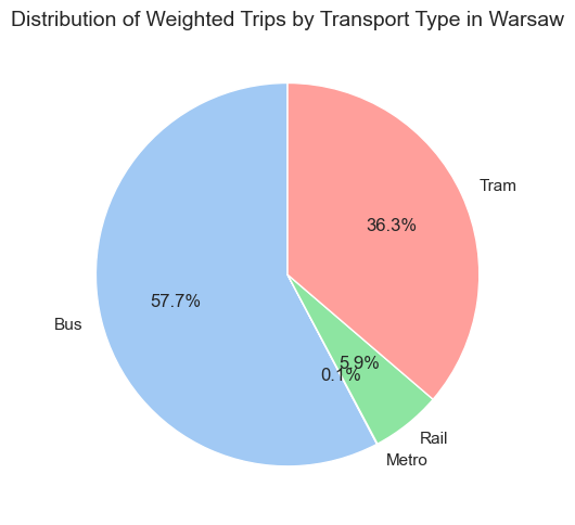
# calculating summary on the weighted impact of each transport type
transport_weighted_totals = aggregated_stops_by_transport.groupby('transport_type')['weighted_trips_capacity'].sum().reset_index()
transport_weighted_totals['share'] = transport_weighted_totals['weighted_trips_capacity'] / transport_weighted_totals['weighted_trips_capacity'].sum()
transport_weighted_totals

	transport_type	weighted_trips_capacity	share
0	Bus	5954584.00	0.58
1	Metro	5210.40	0.00
2	Rail	613147.60	0.06
3	Tram	3742772.00	0.36

# plotting pie chart of weighted trips by transport type
transport_labels = transport_weighted_totals['transport_type'].to_list()

plt.figure(figsize=(5, 5))
plt.pie(
    transport_weighted_totals['weighted_trips_capacity'],
    labels=transport_labels,
    autopct='%1.1f%%',  
    startangle=90,
    shadow=False,  
    colors=sns.color_palette('pastel'))

plt.title('Distribution of Weighted Trips by Transport Type in Warsaw', fontsize=14)
plt.tight_layout()
plt.show();

After recognizing the absence of metro data in the GTFS dataset, we decided to proceed. While we cannot directly compare the impact of transport types from our weighted calculations with official statistics, we can analyze proportions, for example, by comparing the bus to tram ratio in our calculations to that in the official data.

# calculating bus to tram ratios
bus_to_tram_official_stats = 403032807 / 247221160
bus_to_tram_weighted_calc = (transport_weighted_totals.query('transport_type == "Bus"')['weighted_trips_capacity'].sum() 
                             / transport_weighted_totals.query('transport_type == "Tram"')['weighted_trips_capacity'].sum())

# calculating bus to rail ratios
bus_to_rail_official_stats = 403032807 / (17760180 + 30955295 + 3657416) # since the SKM (Suburban Railway) operates like a rail system and is part of Warsaw's broader suburban rail network, it falls under the rail routes category (route_type = 2), not the light rail/tram category. Warsaw Commuter Railway (WKD - Warszawska Kolej Dojazdowa) should be classified under rail routes (route_type = 2), similar to SKM.
bus_to_rail_weighted_calc = (transport_weighted_totals.query('transport_type == "Bus"')['weighted_trips_capacity'].sum() 
                             / transport_weighted_totals.query('transport_type == "Rail"')['weighted_trips_capacity'].sum())

# calculating percentage difference
bus_to_tram_diff = abs((bus_to_tram_weighted_calc - bus_to_tram_official_stats) / bus_to_tram_official_stats) * 100
bus_to_rail_diff = abs((bus_to_rail_weighted_calc - bus_to_rail_official_stats) / bus_to_rail_official_stats) * 100

print(f'Bus to Tram Ratio (Official Statistics): {bus_to_tram_official_stats:.2f}')
print(f'Bus to Tram Ratio (Weighted Calculation): {bus_to_tram_weighted_calc:.2f}')
print(f'Percentage Difference: {bus_to_tram_diff:.2f}%')
print("-"*50)
print(f'Bus to Rail Ratio (Official Statistics): {bus_to_rail_official_stats:.2f}')
print(f'Bus to Rail Ratio (Weighted Calculation): {bus_to_rail_weighted_calc:.2f}')
print(f'Percentage Difference: {bus_to_rail_diff:.2f}%')

Bus to Tram Ratio (Official Statistics): 1.63
Bus to Tram Ratio (Weighted Calculation): 1.59
Percentage Difference: 2.41%
--------------------------------------------------
Bus to Rail Ratio (Official Statistics): 7.70
Bus to Rail Ratio (Weighted Calculation): 9.71
Percentage Difference: 26.20%

Observations

⚠ The calculated proportions are quite close to the official statistics, with differences of 2% (bus to tram) and 31% (bus to rail). Where bus to tram metric is much more meaning for us, since trams represent about 29% of overall traffic while railway transport collectively just for about 6% of overall traffic (thus being much more sensitive for ratio calculation). Therefore, our weighted impact estimations appear reliable enough to trust the analysis and proceed further.

📍 Busiest Stops by Transport Type (Based on Weighted Capacity)

Now we will sort aggregated_stops_by_transport to identify top stops.

# sorting by weighted count to identify top stops
top_weighted_stops_by_transport = (aggregated_stops_by_transport.query('stop_name in @top_20_stops_weighted') # filtering top 20 busiest stops (by weighted capacity)
                                   .sort_values('weighted_trips_capacity', ascending=False))

print('\n\033[1mTop 20 stops (by weighted capacity) with differentiation by transport type:\033[0m')
top_weighted_stops_by_transport

Top 20 stops (by weighted capacity) with differentiation by transport type:

	stop_name	stop_name_central_emoji	transport_type	transport_weight	unique_stop_ids	unique_stop_ids_count	stop_lat_mean	stop_lon_mean	trips_count	weighted_trips_capacity
2187	Rondo Starzyńskiego	Rondo Starzyńskiego 🏙️	Tram	2.20	[100604, 100603, 100608, 100607, 100606, 100605]	6	52.26	21.02	27152	59734.40
398	Dw. Centralny	Dw. Centralny 🏙️	Tram	2.20	[700209, 700210, 700207, 700208]	4	52.23	21.00	20377	44829.40
400	Dw. Gdański	Dw. Gdański 🏙️	Tram	2.20	[701906, 701905, 701907, 701908]	4	52.26	21.00	19066	41945.20
228	Centrum	Centrum 🏙️	Tram	2.20	[701308, 701307, 701309, 701310]	4	52.23	21.01	18550	40810.00
1334	Metro Młociny	Metro Młociny 🌳	Tram	2.20	[605908, 605906, 605905, 605916, 605914, 60592...	9	52.29	20.93	18386	40449.20
1970	Pl. Zawiszy	Pl. Zawiszy 🏙️	Tram	2.20	[400114, 400113, 400105, 400108, 400106]	5	52.23	20.99	17021	37446.20
2661	Wiatraczna	Wiatraczna 🌳	Tram	2.20	[200804, 200812, 200805, 200806, 200807, 20081...	7	52.24	21.08	16811	36984.20
1948	Pl. Narutowicza	Pl. Narutowicza 🏙️	Tram	2.20	[400313, 400311, 400308, 400309, 400312, 40030...	8	52.22	20.98	16282	35820.40
533	Gocławek	Gocławek 🌳	Tram	2.20	[201406, 201403, 201407, 201404, 201405]	5	52.24	21.12	15848	34865.60
1599	Okopowa	Okopowa 🏙️	Tram	2.20	[500304, 500303, 500308, 500307]	4	52.24	20.98	15573	34260.60
1345	Metro Ratusz Arsenał	Metro Ratusz Arsenał 🏙️	Tram	2.20	[709910, 709909, 709904, 709903]	4	52.24	21.00	15496	34091.20
403	Dw. Wileński	Dw. Wileński 🏙️	Tram	2.20	[100303, 100307, 100308]	3	52.25	21.03	15206	33453.20
2191	Rondo Waszyngtona	Rondo Waszyngtona 🏙️	Tram	2.20	[213107, 213108, 213109, 213105, 213106]	5	52.24	21.05	14764	32480.80
1967	Pl. Wilsona	Pl. Wilsona 🌳	Tram	2.20	[600310, 600314, 600313, 600311, 600312]	5	52.27	20.99	13884	30544.80
397	Dw. Centralny	Dw. Centralny 🏙️	Bus	1.00	[700214, 700211, 700202, 700201, 700221, 70021...	14	52.23	21.00	30021	30021.00
876	Kino Femina	Kino Femina 🏙️	Tram	2.20	[708506, 708505, 708509, 708510]	4	52.24	20.99	13641	30010.20
1522	Nowe Bemowo	Nowe Bemowo 🌳	Tram	2.20	[516106, 516104, 516103, 516107, 516108]	5	52.26	20.92	13370	29414.00
874	Kijowska	Kijowska 🏙️	Tram	2.20	[100104, 100106, 100103]	3	52.25	21.04	12485	27467.00
2660	Wiatraczna	Wiatraczna 🌳	Bus	1.00	[200803, 200822, 200808, 200801, 200809, 20081...	11	52.24	21.09	24059	24059.00
21	Al. Zieleniecka	Al. Zieleniecka 🏙️	Tram	2.20	[200106, 200107, 200105]	3	52.25	21.05	10578	23271.60
1937	Pl. Hallera	Pl. Hallera 🏙️	Tram	2.20	[100504, 100503]	2	52.26	21.03	10068	22149.60
1064	Krucza	Krucza 🏙️	Tram	2.20	[703305, 703306]	2	52.23	21.02	9948	21885.60
1333	Metro Młociny	Metro Młociny 🌳	Bus	1.00	[605903, 605901, 605920, 605921, 605904, 60592...	11	52.29	20.93	21562	21562.00
226	Centrum	Centrum 🏙️	Bus	1.00	[701315, 701306, 701304, 701301]	4	52.23	21.01	17257	17257.00
1966	Pl. Wilsona	Pl. Wilsona 🌳	Bus	1.00	[600306, 600309, 600305, 600301, 600307, 60030...	10	52.27	20.99	17042	17042.00
402	Dw. Wileński	Dw. Wileński 🏙️	Bus	1.00	[100301, 100304, 100303, 100309, 100302, 100305]	6	52.25	21.04	15054	15054.00
2190	Rondo Waszyngtona	Rondo Waszyngtona 🏙️	Bus	1.00	[213102, 213101, 213104, 213103]	4	52.24	21.05	14196	14196.00
873	Kijowska	Kijowska 🏙️	Bus	1.00	[100101, 100108, 100107, 100102]	4	52.25	21.04	13394	13394.00
1936	Pl. Hallera	Pl. Hallera 🏙️	Bus	1.00	[100511, 100508, 100507, 100509, 100518, 10050...	8	52.26	21.03	12875	12875.00
20	Al. Zieleniecka	Al. Zieleniecka 🏙️	Bus	1.00	[200109, 200104, 200102, 200101, 200103]	5	52.25	21.05	12011	12011.00
1063	Krucza	Krucza 🏙️	Bus	1.00	[703304, 703303, 703301, 703302]	4	52.23	21.02	11639	11639.00
1969	Pl. Zawiszy	Pl. Zawiszy 🏙️	Bus	1.00	[400102, 400103, 400115, 400104, 400107]	5	52.22	20.99	11446	11446.00
532	Gocławek	Gocławek 🌳	Bus	1.00	[201401, 201402]	2	52.24	21.12	10179	10179.00
399	Dw. Gdański	Dw. Gdański 🏙️	Bus	1.00	[701901, 701902, 701904, 701903]	4	52.26	21.00	6288	6288.00
2186	Rondo Starzyńskiego	Rondo Starzyńskiego 🏙️	Bus	1.00	[100610, 100609, 100612, 100601, 100602]	5	52.26	21.02	6224	6224.00
1521	Nowe Bemowo	Nowe Bemowo 🌳	Bus	1.00	[516110, 516101, 516102, 516115, 516112]	5	52.26	20.92	5827	5827.00
1344	Metro Ratusz Arsenał	Metro Ratusz Arsenał 🏙️	Bus	1.00	[709902, 709901, 709909, 709910, 709906]	5	52.25	21.00	5509	5509.00
875	Kino Femina	Kino Femina 🏙️	Bus	1.00	[708501, 708507, 708502, 708508]	4	52.24	20.99	3974	3974.00
1947	Pl. Narutowicza	Pl. Narutowicza 🏙️	Bus	1.00	[400301, 400302, 400315]	3	52.22	20.98	3838	3838.00
1598	Okopowa	Okopowa 🏙️	Bus	1.00	[500310, 500301, 500302, 500305]	4	52.24	20.98	2836	2836.00
227	Centrum	Centrum 🏙️	Metro	16.70	[7013M:P1]	1	52.23	21.01	8	133.60

Let’s plot a bar chart showing commutative impact of each transport type to stops overall traffic. This time, we’ll again benefit from Plotly’s library, providing great interactivity for visualizations.

# creating a bar plot showing the cumulative impact of each transport type
fig = px.bar(
    top_weighted_stops_by_transport,
    x='weighted_trips_capacity',
    y='stop_name_central_emoji',
    color='transport_type',
    orientation='h',
    title='Top 20 Busiest Stops by Transport Type (by Stop Name and Weighted Trips Capacity) in Warsaw',
    labels={'weighted_trips_capacity': 'Weighted Trips Capacity', 'stop_name_central_emoji': 'Stop Name', 'transport_type':'Transport Type'},
    width=800,
    height=600,
    # category_orders={'stop_name_central_emoji': top_weighted_stops_by_transport},  # sorting bars in the needed order   
    hover_name = 'stop_name_central_emoji',
    hover_data={                         # adding extra data to display at bars selection)
        'trips_count': True,
        'unique_stop_ids_count': True,
        'stop_name_central_emoji':False,
        'stop_lat_mean': ':.4f', 
        'stop_lon_mean': ':.4f' }) 
         
fig.update_layout(
    yaxis={'categoryorder': 'total ascending'},
    title={'x': 0.5, 'y': 0.96}, font=dict(size=14),
    margin=dict(b=105))  # increasing bottom margin for the annotation placement) )

fig.add_annotation(
    text='🏙️ <b>Central stops</b> are within 4 km of the city center (Warsaw Central Station) <br>🌳 <b>Non-central</b> stops are further',
    xref='paper', yref='paper', x=0, y=1.095,
    showarrow=False, font=dict(size=12), align='left')

fig.add_annotation(
    text='<i><b>Note:</b> Weighted Trips Capacity takes into account both trips volume <br>and passengers capacity of different transport serving each stop.</i>',
    xref='paper', yref='paper', x=0, y=-0.25,
    showarrow=False, font=dict(size=12), align='left')

#pio.write_html(fig, file='Top Stops by Transport Type (Bar Plot).html', auto_open=True)
fig.show();

Now we will create a heatmap similar to the previous one but with additional enhancements. It will again highlight the busiest areas in Warsaw, using weighted_trips_capacity values. However, this time, it will also show the impact of each transport type on overall traffic.

Additionally, we will explicitly indicate transport hubs - stations served by two or more transport types (While transport flows through a station do not necessarily mean passengers will enter or exit there, the presence of multiple transport types increases the likelihood of passengers visiting these stops due to line changes).

The map will allow us to select whether to display each transport type and transport hubs.

def create_warsaw_map_by_transport(aggregated_stops_by_transport, multi_transport_stops, title='Warsaw Traffic Map by Public Transport Type'):
    """
    The function creates an interactive map of Warsaw with heatmap and markers differentiated by transport type.
    
    Parameters:
     - aggregated_stops_by_transport (DataFrame): DataFrame containing stop information with transport types
     - multi_transport_stops (DataFrame): DataFrame containing stops that are transportation hubs (serving two and more thasport types)   
     - title (str): title displayig on the map
    
    Returns:
     - folium.Map
    
    Notes:
     - for proper functioning the aggregated_stops_by_transport and multi_transport_stops must contain: `stop_lon_mean`, `stop_lat_mean` and `weighted_trips_capacity`, `stop_name`, `transport_types`, `unique_stop_ids_count`, `trips_count` columns.
     - for proper functioning there must be no missing values in the `stop_lon_mean` and `stop_lat_mean` columns.
    """
    
    city_center = (52.2319, 21.0067)  # latitude and longitude of Warsaw Central Station 
    
    # creating a map centered on Warsaw Central Station 
    warsaw_map = folium.Map(location=city_center, zoom_start=12, tiles='CartoDB positron') #using light-themed map style
   
    # preparing data 
    heat_data = []
    seen_coords = set()
    
    for _, row in aggregated_stops_by_transport.iterrows(): # looping over each row, ignoring indexes returned by iterrows()  
        coord_key = (round(row['stop_lat_mean'], 6), round(row['stop_lon_mean'], 6))
        
          # adding each points only if we haven't seen its coordinates before
        if coord_key not in seen_coords:
            heat_data.append([
                row['stop_lat_mean'], 
                row['stop_lon_mean'], 
                row['weighted_trips_capacity']]) 
            seen_coords.add(coord_key)

    # setting max `weighted_trips_capacity` value for proper scaling
    max_weight = max(point[2] for point in heat_data)

    # creating a heatmap layer 
    heatmap = HeatMap(
        heat_data,
        min_opacity=0.2,
        max_val=max_weight,
        radius=15, 
        blur=15, 
        gradient={'0.4': 'blue', '0.65': 'lime', '0.9': 'orange', '1.0': 'red'}, # converting float keys to strings to avoid AttributeError
        name='Weighted Trips Capacity Heatmap')

    # adding the heatmap to the folium map
    heatmap.add_to(warsaw_map)

    # defining icons for each transport type
    transport_icons = {
        'Bus': 'bus',
        'Tram': 'tram',
        'Metro': 'subway',
        'Rail': 'train'}
        
    # defining colors for each transport type
    transport_colors = {
        'Bus': 'blue',
        'Tram': 'green',
        'Metro': 'red',
        'Rail': 'purple'}

    # creating a marker cluster groups (for interactive points of our transport stops)
    marker_clusters = {}
    for transport_type in aggregated_stops_by_transport['transport_type'].unique():
        marker_clusters[transport_type] = MarkerCluster(name=f"{transport_type} Stops").add_to(warsaw_map)

    for _, row in aggregated_stops_by_transport.iterrows():
        # getting appropriate icons for transport type
        transport_type = row['transport_type']
        icon_name = transport_icons.get(transport_type, 'info-sign')
        icon_color = transport_colors.get(transport_type, 'blue')
        
        # creating popup HTML
        popup_text = f"""
        <b>Stop Name:</b> {row['stop_name']}<br>
        <b>Transport Type:</b> {transport_type}<br>
        <b>Unique Stop IDs Count:</b> {row['unique_stop_ids_count']}<br>
        <b>Trips Count:</b> {row['trips_count']}<br>
        <b>Transport Weight:</b> {row['transport_weight']}<br>
        <b>Weighted Trips Capacity:</b> {row['weighted_trips_capacity']:.0f}
        """
        
        # creating marker and adding directly to appropriate cluster
        folium.Marker(
            location=[row['stop_lat_mean'], row['stop_lon_mean']],
            popup=folium.Popup(popup_text, max_width=300),
            icon=folium.Icon(icon=icon_name, prefix='fa', color=icon_color)
        ).add_to(marker_clusters[transport_type])
    
    # creating a new feature group for transportation hubs
    transport_hubs_layer = folium.FeatureGroup(name="Transportation Hubs 🚩", show=True).add_to(warsaw_map)

    # adding markers for multi-transport stops
    for _, hub in multi_transport_stops.iterrows():
        # Create popup HTML for the hub
        hub_popup_text = f"""
        <b>Hub Name:</b> {hub['stop_name']}<br>
        <b>Transport Types:</b> {hub['transport_types']}<br>
        <b>Unique Stop IDs Count:</b> {hub['unique_stop_ids_count']}<br>
        <b>Trips Count:</b> {hub['trips_count']}<br>
        <b>Weighted Trips Capacity:</b> {hub['weighted_trips_capacity']:.0f}
        """
        
        # creating special icon for hubs
        hub_icon = folium.DivIcon(
            icon_size=(20, 20),
            icon_anchor=(10, 10),
            html=f'<div style="font-size: 18px; color: black;">🚩</div>')
        
        # adding marker to the hubs layer
        folium.Marker(
            location=[hub['stop_lat_mean'], hub['stop_lon_mean']],
            popup=folium.Popup(hub_popup_text, max_width=300),
            icon=hub_icon
        ).add_to(transport_hubs_layer)

    # adding a title to the map
    title_html = f'''
    <div style="position: fixed; 
                top: 5px; left: 50%; transform: translateX(-50%);
                z-index:9999; font-size:14px; font-weight: bold;
                background-color: rgba(255, 255, 255, 0.8); 
                padding: 5px 10px;
                border-radius: 5px; box-shadow: 0 0 2px rgba(0,0,0,0.1);">
        {title}
    </div>
    '''
    
    warsaw_map.get_root().html.add_child(folium.Element(title_html))

    # adding custom legend for heatmap intensity
    legend_html = '''
    <div style="position: fixed; 
                bottom: 20px; right: 10px; width: 190px; 
                border:2px solid grey; z-index:9998; font-size:12px;
                background-color: rgba(255, 255, 255, 0.8); 
                padding: 5px;
                border-radius: 5px;">
        <p style="margin-top: 0;"><b>Heatmap Intensity Scale</b></p>
        <div style="display: flex;">
            <div style="flex-grow: 1; background: linear-gradient(to right, blue, lime, orange, red); height: 15px;"></div>
        </div>
        <div style="display: flex; justify-content: space-between;">
            <span>Low</span>
            <span>Medium</span>
            <span>High</span>
        </div>
        <p style="margin-bottom: 0; font-size: 11px;">Based on Weighted Trips Capacity</p>
        <p style="margin-bottom: 0; font-size: 11px;">Max value: ''' + str(int(max_weight)) + '''</p>
    </div>
    '''

    # adding the legend as an html element to the map
    warsaw_map.get_root().html.add_child(folium.Element(legend_html))
    
    # adding transport type legend
    transport_legend_html = '''
    <div style="position: fixed; 
                bottom: 20px; left: 10px; width: 150px;
                border:2px solid grey; z-index:9998; font-size:12px;
                background-color: rgba(255, 255, 255, 0.8); 
                padding: 5px;
                border-radius: 5px;">
        <p style="margin-top: 0;"><b>Transport Types</b></p>
        <div style="display: flex; align-items: center; margin: 3px 0;">
            <i class="fa fa-bus" style="color: blue; width: 20px; text-align: center;"></i>
            <span style="margin-left: 5px;">Bus</span>
        </div>
        <div style="display: flex; align-items: center; margin: 3px 0;">
            <i class="fa fa-tram" style="color: green; width: 20px; text-align: center;"></i>
            <span style="margin-left: 5px;">Tram</span>
        </div>
        <div style="display: flex; align-items: center; margin: 3px 0;">
            <i class="fa fa-subway" style="color: red; width: 20px; text-align: center;"></i>
            <span style="margin-left: 5px;">Metro</span>
        </div>
        <div style="display: flex; align-items: center; margin: 3px 0;">
            <i class="fa fa-train" style="color: purple; width: 20px; text-align: center;"></i>
            <span style="margin-left: 5px;">Rail</span>
        </div>
        <div style="display: flex; align-items: center; margin: 3px 0;">
            <div style="color: black; width: 20px; text-align: center;">🚩</div>
            <span style="margin-left: 5px;">Transport Hubs</span>
        </div>
    </div>
    '''

    warsaw_map.get_root().html.add_child(folium.Element(transport_legend_html))
    
    # adding a note under the title section
    note_html = '''
    <div style="position: fixed; 
                bottom: 20px; left: 50%; transform: translateX(-50%);
                z-index:9997; font-size:12px; font-style: italic;
                background-color: rgba(255, 255, 255, 0.8); 
                padding: 5px 10px;
                border-radius: 5px; box-shadow: 0 0 2px rgba(0,0,0,0.1);">
        <b>Note:</b> Weighted Trips Capacity takes into account both trips volume and passengers capacity of different transport serving each stop.
    </div>
    '''  
    warsaw_map.get_root().html.add_child(folium.Element(note_html)) 
    
    # adding layer control to choose whether to display different transport types and transport hubs
    folium.LayerControl().add_to(warsaw_map)
    
    return warsaw_map

# finally creating and launching the map
warsaw_map = create_warsaw_map_by_transport(aggregated_stops_by_transport, multi_transport_stops, title="Warsaw Traffic by Transport Type")
warsaw_map

#warsaw_map.save('warsaw_transport_map.html')

Make this Notebook Trusted to load map: File -> Trust Notebook

🎯 Project Summary

• Accomplished Analysis

  • Data sources we used: We analyzed public transport data using reliable sources, including official reports from Warsaw’s transport authorities (e.g., ZTM Report 2022). Our main dataset was GTFS data for Warsaw, last updated on January 18, 2025. This data, covering a two month period, was considered accurate and sufficient for our study.

  • Checking data quality and preparation for further analysis: We checked the data and no critical issues like duplicates or missing values in key fields were revealed. However, we noted a lack of comprehensive metro data, as only a few records were included. Necessary table merges were performed to link and prepare the data for analysis.

  • Passenger flow estimation: To better represent traffic, we calculated weighted trips capacity by combining trip counts with average transport capacity per type. We verified our approach by comparing our figures with the official statistics, they align pretty well.
    

  • Visualizations:

    • We identified the busiest stops and displayed them in interactive bar plots showing:
      • Trips count per stop id.
      • Trips count per stop name (that may contain several stop ids).
      • Weighted trips capacity per stop name.
      • Weighted trips capacity per stop name by transport type.
        
      • We highlighted non-central stations, as we focused on them (we defined central stations as those within 4 km from Warsaw Central Railway station and distinguished them from others). Thanks to Plotly library, these visualizations are very interactive and allow to explore additional details associated with each stop (like transport types, coordinates and trips number).
    • Two detailed interactive maps were created using Folium:
      • The heatmap showing weighted trips capacity and overall information on stops without separation by transport types.
        • This map is best for visualizing aggregated passenger flows (regardless of transport types) and high-traffic areas.
      • The layered map visualizing how different transport types contribute to traffic. It also explicitly demonstrates transport hubs (stations served by two or more transport types, that likely demonstrate higher passenger activity).
        • This map is best for analyzing how each transport type contributes to overall traffic, it also highlights transport hubs (stations with multiple transport types) that tend to have higher passenger activity because of their connections.
• Next Steps

  • Addressing metro data gaps: The GTFS data we used lacks metro coverage. We can retrieve data from platforms like the Warsaw Open Data Portal or directly from metro authorities (if possible). This would improve our passenger flow estimates by about 19% (based on official metro traffic stats).

  • Time-based analysis: GTFS data allows us to analyze traffic by time intervals, revealing daily and hourly trends. We can make needed calculations and add temporal layer to our analyses (even on the heatmaps) this would help better choose pizzeria locations and operating hours.

  • Adding car traffic: We found reliable traffic data from the Municipal Roads Authority (2022) (link here). Including this data would provide another layer for insights on people flows.

📋 References

• Official reports

  1. ZTM Report 2022 - This is the original report by the Public Transport Authority (Zarząd Transportu Miejskiego) detailing Warsaw’s public transportation system’s performance and statistics for 2022.
  2. WARSAW PUBLIC TRANSPORT AUTHORITY, REPORT 2022 (Archived version; the original site ztm.waw.pl was unavailable during the study) - This is the revised report by the Public Transport Authority (Zarząd Transportu Miejskiego) for 2022. Note: The archived version has “popr” in the filename, indicating “poprawiony” (corrected) in Polish, suggesting that this report might be a revised version of the original.
  3. ANNUAL REPORT: PUBLIC ROADS AUTHORITY IN WARSAW 2022 - This report by the Public Roads Authority in Warsaw (ZDM - Zarząd Dróg Miejskich) provides information about road infrastructure, traffic management, and related data within Warsaw for 2022.
  4. MUNICIPAL ROADS AUTHORITY - Automatic Traffic Measurement Results (2022) - This interactive map and set of tables presents average daily vehicle traffic data for 2022, as provided by the Municipal Roads Authority.

• Data sources

  5. GTFS Data for Warsaw (mkuran.pl) - GTFS (General Transit Feed Specification) data for Warsaw, providing a standardized format for public transportation schedules and related geographic data.
  6. Warsaw open data portal (Not directly utilized in this study but highlighted as a valuable resource for future analyses) - The official Warsaw open data portal that offers various datasets related to the city.

• Public transport operators and company websites

  7. The website of the Office of Rail Transport (Strona Urzędu Transportu Kolejowego) - The official website of the Office of Rail Transport in Poland, offering information about rail transport regulations and statistics.
  8. City of Warsaw’s official portal - Urban Transport - The official website of the City of Warsaw that provides information about urban transport services.
  9. Metro Warszawskie - Company Profile, including expansion plans - A section of the official Warsaw Metro website offering company information, including rolling stock details and expansion plans.
  10. Metro Warszawskie Sp. z o. o - Official Website - The official website of the Warsaw Metro operator.

• Research and studies on public transport in warsaw

  11. Analysis of Accessibility of Public Transport in Warsaw in the Opinion of Users - A research paper analyzing the accessibility of public transport in Warsaw based on user feedback.
  12. Study: Measuring Dynamic Public Transit Accessibility to Local Centres in Warsaw - A study measuring dynamic public transit accessibility to local centers in Warsaw.

• Wikipedia and general reference pages

  13. General Transit Feed Specification - The official documentation for the General Transit Feed Specification (GTFS).
  14. Wikipedia: Warsaw Public Transport
  15. Wikipedia: Warsaw Metro
  16. Wikipedia: Transport in Warsaw

Note: Some of the sources may require a VPN with the country set to Poland to access them. And some sources may require translation from Polish.